Law of the single logarithm for randomly weighted sums of dependent sequences and an application

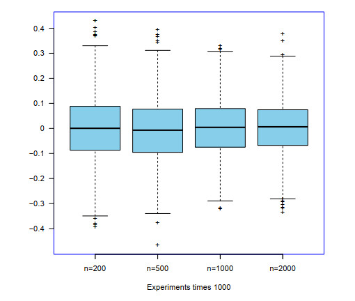
1.   Introduction

With the development of information technology, the datasets with lots of features have been collected in many application fields. However, datasets usually contain many redundant features, which may affect the classification ability of datasets and increase the complexity of learning algorithms. Feature selection is a data preprocessing technology which selects a subset from the original feature set to improve the performance of learning algorithms. So far, feature selection has been applied to rule extraction ^[1], decision-making ^[4,24], and data mining ^[30].

Rough set theory ^[12] is a typical granular computing model and a meaningful mathematical tool for feature selection, which is also called attribute reduction in rough set theory. In rough set theory, the datasets are represented as information systems. Due to the diversity of the datasets, different types of information systems are discussed, whose attribute reduction structures are explored by different rough set models. For example, the attribute reduction of a complete decision information system (CDIS) was investigated based on the classical Pawlak rough set model, which is defined by equivalence (indiscernibility) relations or partitions^[13,16,31]. The attribute reduction of an incomplete decision information system (IDIS) was discussed by relation rough sets^[3,9,17,23]. The neighborhood rough set model, defined on neighborhood granularies, was used to attribute reduction of neighborhood DISs^[5,6,33]. The covering rough sets defined on coverings were utilized for reducing covering DISs ^[2,22,25,26]. The rough set models mentioned above are constructed by a single granular knowledge. However, in real-world applications, more and more datasets should be described via multiple granular structures. Qian et al. proposed the concepts of multi-granulation rough sets in CDISs and discussed attribute reduction of CDISs based on multi-granulation rough sets ^[14,18]. Kong et al. explored multi-granulation reduction of information systems ^[8]. Attribute reduction of IDISs based on multi-granulation rough sets was explored in ^[15]. Zhang et al. defined a generalized multi-granulation fuzzy neighborhood rough set model and discussed a feature selection method by the model ^[34].

The technique of constructing discernibility matrices and discernibility functions, proposed by Skowron and Rauszer ^[20] and Skowron ^[19], is an important attribute reduction method. Yao and Zhao defined a minimal family of discernibility sets based on the family of discernibility sets to compute the reducts of CDISs ^[29]. Zhao et al. constructed the relative discernibility matrix of a CDIS to get relative reducts^[35]. Jiang and Yu proposed a compactness discernibility information tree to obtain the minimal attribute reduction of a CDIS ^[7]. Ma et al. introduced a compressed binary discernibility matrix and designed an incremental attribute reduction algorithm for getting an attribute reduction set of a dynamic CDIS ^[10]. A binary discernibility matrix was designed to get attribute relative reducts of an IDIS ^[11]. Chen et al. ^[2], Wang et al. ^[22] and Yang et al. ^[25] constructed discernibility matrices to obtain the reducts of covering DISs. The discernibility techniques are also used to achieve the knowledge reduction of information systems based on multi-granulation rough sets. Tan et al. constructed discenibility matrices and discernibility functions to calculate the attribute reducts of a decision multi-granulation space (DMS) ^[21] and verified the effectiveness of the reduction methods by numerical experiments. However, the optimistic lower reducts are not calculated by discenibility matrices in ^[21]. Zhang et al. explored the attribute reduction of an IDIS by the discernibility approach in multi-granulation rough set theory ^[32] and presented numerical experiments to show the feasibility and effectiveness of the algorithms to get reducts. However, the attribute reduction of IDISs based on optimistic multi-granulation rough sets is not considered in ^[32].

The purpose of this paper is to analyze and compare the multi-granulation reduction theory of DMSs ^[21] and IDISs ^[32] from discernibility, and to present a general model for the multi-granulation reduction of DISs by the discernibility technique, which can provide a theoretical basis for the multi-granulation reduction of DISs based on discernibility. The notation of a GNDIS is introduced in this paper, the multi-granulation reductions of GNDISs based on the multi-granulation rough set are discussed, and discernibility matrices are constructed to compute the multi-granulation reducts of GNDISs. Then, the pessimistic (or optimistic) approximations in DMSs and IDISs can be changed into the multi-granulation pessimistic (or optimistic) approximations in GNDISs. Moreover, the pessimistic multi-granulation reducts and the optimistic multi-granulation reducts of DMSs discussed in ^[21] can be computed by the discernibility matrices and discernibility functions based on the multi-granulation reduction theory of GNDISs. Additionally, the pessimistic multi-granulation reduction structures of IDISs discussed in ^[32] are characterized by the reduction theory of GNDISs based on discernibility technique.

The remaining structure of this paper is organized as follows. In Section 2, the definitions about multi-granulation rough sets are reviewed. In Section 3, we introduce the definition of the multi-granulation rough sets in a GNDIS and discuss knowledge reduction of a GNDIS based on the multi-granulation rough sets. The discernibility matrices and discernibility functions are constructed to characterize the multi-granulation reducts of a GNDIS. In Section 4, relationships between the multi-granulation reduction of DMSs and that of GNDISs are discussed. Moreover, the optimistic lower reducts of DMSs are discussed by the discernibility matrices in this section. Section 5 explores relationships between the multi-granulation reduction of IDISs and that of GNDISs. Then, the optimistic multi-granulation reductions of IDISs from the discernibility technique are presented in this section. Section 6 concludes this study.

2.   Preliminary knowledge on multi-granulation rough sets

In this section, we review some basic concepts about multi-granulation rough sets, which were proposed by Qian et al. ^[18] to approximate a target concept using multiple binary relations.

2.1.   Multi-granulation rough sets in DMSs

Suppose that $(U, A, d)$ is a DIS, in which $U$ is the universe, $A$ is a family of condition attributes where $a:U\rightarrow V_{a}$ for any $a\in A$, $V_{a}$ is the value set of $a$, and $d:U\rightarrow V_{d}$ is a decision attribute where $V_{d}$ is the value set of $d$.

In a DIS $(U, A, d)$, $\mathcal{A} = \{A_{k}|A_{k}\subseteq A, k = 1, 2, \cdots, m\}$ is a family of attribute subsets. Then, $(U, \mathcal{A}, d)$ is called an DMS ^[28]. Each $A_{k}\in \mathcal{A}$ induces an equivalent relation $R_{A_{k}} = \{(x, y)\in U\times U|\forall a\in A_{k}(a(x) = a(y))\}$ and generates a granular structure $U/R_{A_{k}} = \{[x]_{A_{k}}|x\in U\}$, in which $[x]_{A_{k}} = \{y\in U|(x, y)\in R_{A_{k}}\}$. The decision attribute $d$ generates a partition $U/R_{d} = \{[x]_{d}|x\in U\}\triangleq\{X_{1}, X_{2}, \cdots, X_{n}\}$, each of which is the decision class with the same decision attribute values. The pessimistic multi-granulation lower and upper approximations and optimistic multi-granulation lower and upper approximations were discussed by Qian et al.^[14,18].

Definition 1. ^[14] Given a DMS $(U, \mathcal{A}, d)$ with $\mathcal{A} = \{A_{k}\subseteq A|k\in\mathbb{Z}, 1\leq k \leq m\}$, let $X\subseteq U$. Define the pessimistic multi-granulation lower and upper approximations of $X$ as

$\underline{\sum\limits_{\mathcal{A}} A_{k}^{P}}(X) = \{x\in U|([x]_{A_{1}}\subseteq X) \wedge ([x]_{A_{2}}\subseteq X) \wedge \cdots \wedge ([x]_{A_{m}}\subseteq X)\}$,

$\overline{\sum\limits_{\mathcal{A}} A_{k}^{P}}(X) = \sim\underline{\sum\limits_{\mathcal{A}} A_{k}^{P}}(\sim X)$.

One calls ($\underline{\sum\limits_{\mathcal{A}} A_{k}^{P}}(X)$, $\overline{\sum\limits_{\mathcal{A}} A_{k}^{P}}(X)$) a pessimistic multi-granulation rough set.

For each $x\in U$, $\mathcal{H}\subseteq \mathcal{A}$, denote $\cup_{A\in \mathcal{H}}[x]_{A}$ by $N_{\mathcal{H}}(x)$. Then, it is easy to get that $\underline{\sum\limits_{\mathcal{A}} A_{k}^{P}}(X) = \{x\in U|N_{\mathcal{A}}(x)\subseteq U\}$.

Definition 2. ^[18] Given a DMS $(U, \mathcal{A}, d)$ with $\mathcal{A} = \{A_{k}\subseteq A|k\in\mathbb{Z}, 1\leq k \leq m\}$, let $X\subseteq U$. Define the optimistic multi-granulation lower and upper approximations of $X$ as

$\underline{\sum\limits_{\mathcal{A}} A_{k}^{O}}(X) = \{x\in U|([x]_{A_{1}}\subseteq X) \vee ([x]_{A_{2}}\subseteq X) \vee \cdots \vee ([x]_{A_{m}}\subseteq X)\}$,

$\overline{\sum\limits_{\mathcal{A}} A_{k}^{O}}(X) = \sim\underline{\sum\limits_{\mathcal{A}} A_{k}^{O}}(\sim X)$.

($\underline{\sum\limits_{\mathcal{A}} A_{k}^{P}}(X)$, $\overline{\sum\limits_{\mathcal{A}} A_{k}^{P}}(X)$) is called an optimistic multi-granulation rough set.

2.2.   Multi-granulation rough sets in IDISs

If some attribute values of attributes in $A$ of a DIS $(U, A, d)$ are are missing or unknown, then the missing attribute value is expressed by special symbol '$\ast$' and $(U, A, d)$ is termed as an IDIS. For any $A_{k}\subseteq A$, a tolerance relation is defined by Kryszkiewicz as ^[9]:

$SIM(A_{k}) = \{(x, y)\in U\times U|\forall a\in A_{k}(a(x) = a(y)\vee a(x) = \ast \vee a(y) = \ast)\}$.

A granular structure is induced by $A_{k}$ as $U/SIM(A_{k}) = \{S_{A_{k}}(x) |x\in U\}$, where $S_{A_{k}}(x) = \{y\in U|(x, y)\in SIM(A_{k})\}$.

The multi-granulation rough sets in IDISs were introduced by Qian et al. ^[15].

Definition 3. ^[15] Given an IDIS $(U, A, d)$ with $\mathcal{A}^{I} = \{A_{k}\subseteq A|k\in\mathbb{Z}, 1\leq k \leq m\}$, let $X\subseteq U$. Define the pessimistic multi-granulation lower and upper approximations of $X$ as

$\underline{\sum\limits_{\mathcal{A}^{I}} A_{k}^{P}}(X) = \{x\in U|(S_{A_{1}}(x)\subseteq X) \wedge (S_{A_{2}}(x)\subseteq X) \wedge \cdots \wedge (S_{A_{m}}(x)\subseteq X)\}$,

$\overline{\sum\limits_{\mathcal{A}^{I}} A_{k}^{P}}(X) = \sim\underline{\sum\limits_{\mathcal{A}^{I}} A_{k}^{P}}(\sim X)$.

Define the optimistic multi-granulation lower and upper approximations of $X$

$\underline{\sum\limits_{\mathcal{A}^{I}} A_{k}^{O}}(X) = \{x\in U|(S_{A_{1}}(x)\subseteq X) \vee (S_{A_{2}}(x)\subseteq X) \vee \cdots \vee (S_{A_{m}}(x)\subseteq X)\}$,

$\overline{\sum\limits_{\mathcal{A}^{I}} A_{k}^{O}}(X) = \sim\underline{\sum\limits_{\mathcal{A}^{I}} A_{k}^{O}}(\sim X)$.

$(\underline{\sum\limits_{\mathcal{A}^{I}} A_{k}^{P}}(X), \overline{\sum\limits_{\mathcal{A}^{I}} A_{k}^{P}}(X))$ and $(\underline{\sum\limits_{\mathcal{A}^{I}} A_{k}^{O}}(X), \overline{\sum\limits_{\mathcal{A}^{I}} A_{k}^{O}}(X))$ are, respectively, the pessimistic multi-granulation rough set and optimistic multi-granulation rough set of $X$.

For each $x\in U$, $\mathcal{H}\subseteq \mathcal{A}^{I}$, denote $\cup_{A\in \mathcal{H}}S_{A}(x)$ by $IN_{\mathcal{H}}(x)$. It is clear that $\underline{\sum\limits_{\mathcal{A}^{I}} A_{k}^{P}}(X) = \{x\in U|IN_{\mathcal{A}^{I}}(x)\subseteq U\}$.

3.   Multi-granulation reduction of GNDISs

In this section, we present the definitions of multi-granulation rough sets in GNDISs and explore multi-granulation reduction of GNDISs. Throughout this paper, the universe of discourse $U$ is nonempty and finite. The family of all subsets of $U$ is denoted by $\mathcal{P}(U)$. For $X\subseteq U$, $\sim X$ is the complementary set of $X$.

3.1.   Multi-granulation rough sets in GNDISs

Some basic concepts about the neighborhood operator is presented in ^[27].

Definition 4. ^[27] Let $U$ be the universe. A mapping $N:U\rightarrow \mathcal{P}(U)$ is called a neighborhood operator. If $x \in N(x)$ for all $x \in U$, $N$ is a reflexive neighborhood operator. If $x \in N(y)\Rightarrow y\in N(x)$ for all $x, y \in U$, $N$ is a symmetric neighborhood operator. If $[y \in N(x), z\in N(y)]\Rightarrow z\in N(x)$ for all $x, y, z \in U$, $N$ is a transitive neighborhood operator. If the neighborhood operator $N$ is reflexive, symmetric and transitive, $N$ is called a Pawlak neighborhood operator.

Clearly, $\{N(x)|x\in U\}$ of a Pawlak neighborhood operator $N$ forms a partition of $U$.

Definition 5. Let $N$ be a reflexive neighborhood operator on $U$. Denote $\{N(x)|x\in U\}$ by $C_{N}$. The ordered pair $(U, N)$ is called a generalized neighborhood approximation space.

Clearly, $C_{N}$ from $(U, N)$ is a covering. We introduce the generalized neighborhood multi-granulation rough sets now.

Definition 6. Let $N_{1}, N_{2}, \cdots, N_{m}(m\geq 2)$ be reflexive neighborhood operators on $U$ and $\mathcal{N} = \{N_{1}, N_{2}, \cdots$, $N_{m}\}$, $N_{d}:U\rightarrow P(U)$ be a Pawlak neighborhood operator, then $(U, \mathcal{N}, N_{d})$ is called a GNDIS. For $X\subseteq U$, define the generalized neighborhood pessimistic lower approximation $\underline{\sum\limits_{\mathcal{N}} N_{k}^{P}}(X)$ and pessimistic upper approximation $\overline{\sum\limits_{\mathcal{N}} N_{k}^{P}}(X)$ by

$\underline{\sum\limits_{\mathcal{N}} N_{k}^{P}}(X) = \{x\in U|(N_{1}(x)\subseteq X) \wedge (N_{2}(x)\subseteq X) \wedge \cdots \wedge(N_{m}(x)\subseteq X)\}$,

$\overline{\sum\limits_{\mathcal{N}} N_{k}^{P}}(X) = \sim\underline{\sum\limits_{\mathcal{N}} N_{k}^{P}}(\sim X)$.

$(\underline{\sum\limits_{\mathcal{N}} N_{k}^{P}}(X), \overline{\sum\limits_{\mathcal{N}} N_{k}^{P}}(X))$ is the generalized neighborhood pessimistic multi-granulation rough set of $X$.

For $\mathcal{H}\subseteq \mathcal{N}$ and $x\in U$, denote $GN_{\mathcal{H}}(x) = \bigcup_{N\in\mathcal{H}}N(x)$. Then, it is clear that $\underline{\sum\limits_{\mathcal{N}} N_{k}^{P}}(X) = \{x\in U|GN_{\mathcal{N}}(x) \subseteq X\}$.

Proposition 1. Let $(U, \mathcal{N}, N_{d})$ be a GNDIS, $X, Y\subseteq U$, $\mathcal{H}\subseteq\mathcal{N}$ and $\mathcal{H}\neq\emptyset$, then:

(1) $\underline{\sum\limits_{\mathcal{N}} N_{k}^{P}}(\emptyset) = \emptyset$, $\underline{\sum\limits_{\mathcal{N}} N_{k}^{P}}(U) = U$, $\overline{\sum\limits_{\mathcal{N}}N_{k}^{P}}(\emptyset) = \emptyset$, $\overline{\sum\limits_{\mathcal{N}} N_{k}^{P}}(U) = U$.

(2) $\underline{\sum\limits_{\mathcal{N}} N_{k}^{P}}(X)\subseteq X \subseteq \overline{\sum\limits_{\mathcal{N}} N_{k}^{P}}(X)$.

(3) $X\subseteq Y \; \Rightarrow \; \underline{\sum\limits_{\mathcal{N}} N_{k}^{P}}(X)\subseteq \underline{\sum\limits_{\mathcal{N}} N_{k}^{P}}(Y)$, $\overline{\sum\limits_{\mathcal{N}}N_{k}^{P}}(X)\subseteq \overline{\sum\limits_{\mathcal{N}} N_{k}^{P}}(Y)$.

(4) $\underline{\sum\limits_{\mathcal{N}} N_{k}^{P}}(X\cap Y) = \underline{\sum\limits_{\mathcal{N}} N_{k}^{P}}(X)\cap \underline{\sum\limits_{\mathcal{N}} N_{k}^{P}}(Y)$, $\overline{\sum\limits_{\mathcal{N}} N_{k}^{P}}(X\cup Y) = \overline{\sum\limits_{\mathcal{N}} N_{k}^{P}}(X)\cup\overline{\sum\limits_{\mathcal{N}} N_{k}^{P}}(Y)$.

(5) $\underline{\sum\limits_{\mathcal{N}} N_{k}^{P}}(\underline{\sum\limits_{\mathcal{N}} N_{k}^{P}}(X))\subseteq \underline{\sum\limits_{\mathcal{N}} N_{k}^{P}}(X)$, $\overline{\sum\limits_{\mathcal{N}} N_{k}^{P}}(X)\subseteq \overline{\sum\limits_{\mathcal{N}} N_{k}^{P}}(\overline{\sum\limits_{\mathcal{N}} N_{k}^{P}}(X))$.

(6) $\underline{\sum\limits_{\mathcal{N}} N_{k}^{P}}(X)\subseteq \underline{\sum\limits_{\mathcal{H}} N_{k}^{P}}(X)$, $\overline{\sum\limits_{\mathcal{H}} N_{k}^{P}}(X)\subseteq \overline{\sum\limits_{\mathcal{N}} N_{k}^{P}}(X)$.

Proof. It is verified by Definition 6. □

Definition 7. Given a GNDIS $(U, \mathcal{N}, N_{d})$ with $\mathcal{N} = \{N_{1}, N_{2}, \; \cdots, N_{m}\}$, let $X\subseteq U$. Define the generalized neighborhood optimistic lower approximation $\underline{\sum\limits_{\mathcal{N}} N_{k}^{O}}(X)$ and optimistic upper approximation $\overline{\sum\limits_{\mathcal{N}} N_{k}^{O}}(X)$ of $X$ as

$\underline{\sum\limits_{\mathcal{N}} N_{k}^{O}}(X) = \{x\in U|(N_{1}(x)\subseteq X) \vee (N_{2}(x)\subseteq X) \vee \cdots \vee (N_{m}(x)\subseteq X)\}$,

$\overline{\sum\limits_{\mathcal{N}} N_{k}^{O}}(X) = \sim\underline{\sum\limits_{\mathcal{N}} N_{k}^{O}}(\sim X)$.

$(\underline{\sum\limits_{\mathcal{N}} N_{k}^{O}}(X), \overline{\sum\limits_{\mathcal{N}} N_{k}^{O}}(X))$ is the generalized neighborhood optimistic multi-granulation rough set of $X$.

Proposition 2. Let $(U, \mathcal{N}, N_{d})$ be a GNDIS, $X, Y\subseteq U$, $\mathcal{H}\subseteq\mathcal{N}$ and $\mathcal{H}\neq\emptyset$, then:

(1) $\underline{\sum\limits_{\mathcal{N}} N_{k}^{O}}(\emptyset) = \emptyset$, $\underline{\sum\limits_{\mathcal{N}} N_{k}^{O}}(U) = U$, $\overline{\sum\limits_{\mathcal{N}} N_{k}^{O}}(\emptyset) = \emptyset$, $\overline{\sum\limits_{\mathcal{N}} N_{k}^{O}}(U) = U$.

(2) $\underline{\sum\limits_{\mathcal{N}} N_{k}^{O}}(X)\subseteq X \subseteq \overline{\sum\limits_{\mathcal{N}} N_{k}^{O}}(X)$.

(3) $X\subseteq Y \; \Rightarrow \; \underline{\sum\limits_{\mathcal{N}} N_{k}^{O}}(X)\subseteq \underline{\sum\limits_{\mathcal{N}} N_{k}^{O}}(Y)$, $\overline{\sum\limits_{\mathcal{N}} N_{k}^{O}}(X)\subseteq \overline{\sum\limits_{\mathcal{N}} N_{k}^{O}}(Y)$.

(4) $\underline{\sum\limits_{\mathcal{N}} N_{k}^{O}}(X\cap Y)\subseteq\underline{\sum\limits_{\mathcal{N}} N_{k}^{O}}(X)\cap \underline{\sum\limits_{\mathcal{N}} N_{k}^{O}}(Y)$, $\overline{\sum\limits_{\mathcal{N}} N_{k}^{O}}(X)\cup\overline{\sum\limits_{\mathcal{N}} N_{k}^{O}}(Y)\subseteq\overline{\sum\limits_{\mathcal{N}} N_{k}^{O}}(X\cup Y)$.

(5) $\underline{\sum\limits_{\mathcal{N}} N_{k}^{O}}(\underline{\sum\limits_{\mathcal{N}} N_{k}^{O}}(X))\subseteq \underline{\sum\limits_{\mathcal{N}} N_{k}^{O}}(X)$, $\overline{\sum\limits_{\mathcal{N}} N_{k}^{O}}(X)\subseteq \overline{\sum\limits_{\mathcal{N}} N_{k}^{O}}(\overline{\sum\limits_{\mathcal{N}} N_{k}^{O}}(X))$.

(6) $\underline{\sum\limits_{\mathcal{H}} N_{k}^{O}}(X)\subseteq \underline{\sum\limits_{\mathcal{N}} N_{k}^{O}}(X)$, $\overline{\sum\limits_{\mathcal{N}} N_{k}^{O}}(X)\subseteq\overline{\sum\limits_{\mathcal{H}} N_{k}^{O}}(X)$.

Proof. It is easy to obtain the conclusion by Definition 7. □

3.2.   Pessimistic multi-granulation reduction of GNDISs

In a GNDIS $(U, \mathcal{N}, N_{d})$, $C_{N_{d}} = \{N_{d}(y)|y\in U\}$ is a partition of $U$. In the following, the GNDIS mentioned satisfies $|C_{N_{d}}|\geq 2$. In this subsection, we present pessimistic multi-granulation reduction of GNDISs.

Definition 8. Given a GNDIS $(U, \mathcal{N}, N_{d})$, let $\mathcal{H} \subseteq \mathcal{N}$.

(1) If $\underline{\sum\limits_{\mathcal{N}} N_{k}^{P}}(N_{d}(y)) = \underline{\sum\limits_{\mathcal{H}} N_{k}^{P}}(N_{d}(y))$ for all $y\in U$, then we say that $\mathcal{H}$ is a generalized neighborhood pessimistic lower consistent set (GNPL-consistent set). Denote the family of all GNPL-consistent sets by $Cons_{L}^{P}(\mathcal{N})$. If $\mathcal{H}\in Cons_{L}^{P}(\mathcal{N})$, and $\mathcal{H}^{\prime}\not\in Cons_{L}^{P}(\mathcal{N})$ whenever $\mathcal{H}^{\prime}\subset\mathcal{H}$, then $\mathcal{H}$ is called a GNPL-reduct. Denote the set of all GNPL-reducts by $Red_{L}^{P}(\mathcal{N})$, the core w.r.t. GNPL-reducts is defined as $Core_{L}^{P}(\mathcal{N}) = \bigcap\{\mathcal{H}|\mathcal{H}\in Red_{L}^{P}(\mathcal{N})\}$.

(2) If $\overline{\sum\limits_{\mathcal{N}} N_{k}^{P}}(N_{d}(y)) = \overline{\sum\limits_{\mathcal{H}} N_{k}^{P}}(N_{d}(y))$ for all $y\in U$, then we say that $\mathcal{H}$ is a generalized neighborhood pessimistic upper consistent set (GNPU-consistent set). Denote the family of all GNPU-consistent sets by $Cons_{U}^{P}(\mathcal{N})$. If $\mathcal{H}\in Cons_{U}^{P}(\mathcal{N})$, and $\mathcal{H}^{\prime}\not\in Cons_{U}^{P}(\mathcal{N})$ whenever $\mathcal{H}^{\prime}\subset\mathcal{H}$, then $\mathcal{H}$ is called a GNPU-reduct. Denote the set of all GNPU-reducts as $Red_{U}^{P}(\mathcal{N})$, the core w.r.t. GNPU-reducts is defined by $Core_{U}^{P}(\mathcal{N}) = \bigcap\{\mathcal{H}|\mathcal{H}\in Red_{U}^{P}(\mathcal{N})\}$.

From Definition 8, we can see that a GNPL-reduct (or a GNPU-reduct) is a minimal subset of $\mathcal{N}$, which preserves the pessimistic lower approximations (or the pessimistic upper approximations) of all sets in $C_{N_{d}}$. The pessimistic lower and upper reducts of a GNDIS are different, which are illustrated by an example in the following.

Example 1. (1) A GNDIS $(U, \mathcal{N}, N_{d})$ is presented in Table 1, where $U = \{x_{1}, x_{2}, \cdots, x_{6}\}$ and $\mathcal{N} = \{N_{1}, N_{2}, \cdots, N_{5}\}$. The generalized neighborhood granules of $x\in U$ are presented in Table 2.

By Definition 6, we get that $\underline{\sum\limits_{\mathcal{N}}N_{k}^{P}}(\{x_{1}, x_{2}, x_{3}\}) = \{x_{1}\}$, $\underline{\sum\limits_{\mathcal{N}}N_{k}^{P}}(\{x_{4}, x_{5}\}) = \emptyset$, $\underline{\sum\limits_{\mathcal{N}}N_{k}^{P}}(\{x_{6}\}) = \emptyset$, $\overline{\sum\limits_{\mathcal{N}}N_{k}^{P}}(\{x_{1}, x_{2}, x_{3}\}) = U$, $\overline{\sum\limits_{\mathcal{N}}N_{k}^{P}}(\{x_{4}, x_{5}\}) = \{x_{2}, x_{3}, x_{4}, x_{5}\}$, $\overline{\sum\limits_{\mathcal{N}}N_{k}^{P}}(\{x_{6}\}) = \{x_{3}, x_{6}\}$.

Let $\mathcal{H} = \{N_{3}, N_{4}\}$. We compute that $\underline{\sum\limits_{\mathcal{H}}N_{k}^{P}}(N_{d}(x_{i})) = \underline{\sum\limits_{\mathcal{N}}N_{k}^{P}}(N_{d}(x_{i}))$ for $i = 1, 2, \cdots, 6$. Thus, $\mathcal{H}$ is a GNPL-consistent set. Let $\mathcal{H}_{1} = \{N_{3}\}$. We get that $\underline{\sum\limits_{\mathcal{H}_{1}}N_{k}^{P}}(\{x_{4}, x_{5}\}) = \{x_{5}\}\neq\underline{\sum\limits_{\mathcal{N}}N_{k}^{P}}(\{x_{4}, x_{5}\})$, which follows that $\mathcal{H}_{1}$ is not a GNPL-consistent set. Let $\mathcal{H}_{2} = \{N_{4}\}$. We obtain that $\underline{\sum\limits_{\mathcal{H}_{2}}N_{k}^{P}}(\{x_{1}, x_{2}, x_{3}\}) = \{x_{1}, x_{2}, x_{3}\}\neq\underline{\sum\limits_{\mathcal{N}}N_{k}^{P}}(\{x_{1}, x_{2}, x_{3}\})$, which implies that $\mathcal{H}_{2}$ is not a GNPL-consistent set. So $\mathcal{H}$ is a GNPL-reduct. Due to $\overline{\sum\limits_{\mathcal{H}}N_{k}^{P}}(\{x_{4}, x_{5}\}) = \{x_{2}, x_{4}, x_{5}\}\neq \overline{\sum\limits_{\mathcal{N}}N_{k}^{P}}(\{x_{4}, x_{5}\})$, $\mathcal{H}$ is not a GNPU-consistent set, then $\mathcal{H}$ is not a GNPU-reduct. At the same time, we get a conclusion: A GNPL-reduct is not necessarily a GNPU-reduct.

(2) The operator $N_{d}:U\rightarrow P(U)$ in (1) is changed by: $N_{d}(x_{1}) = N_{d}(x_{2}) = N_{d}(x_{3}) = \{x_{1}, x_{2}, x_{3}\}$, $N_{d}(x_{4}) = N_{d}(x_{5}) = N_{d}(x_{6}) = \{x_{4}, x_{5}, x_{6}\}$. Then, we get another GNDIS $(U, \mathcal{N}, N_{d})$. By Definition 6, we have that $\underline{\sum\limits_{\mathcal{N}}N_{k}^{P}}(\{x_{1}, x_{2}, x_{3}\}) = \{x_{1}\}$, $\underline{\sum\limits_{\mathcal{N}}N_{k}^{P}}(\{x_{4}, x_{5}, x_{6}\}) = \emptyset$, $\overline{\sum\limits_{\mathcal{N}}N_{k}^{P}}(\{x_{1}, x_{2}, x_{3}\}) = U$, $\overline{\sum\limits_{\mathcal{N}}N_{k}^{P}}(\{x_{4}, x_{5}, x_{6}\}) = \{x_{2}, x_{3}, x_{4}, x_{5}, x_{6}\}$.

Let $\mathcal{H} = \{N_{2}\}$. We obtain that $\overline{\sum\limits_{\mathcal{H}}N_{k}^{P}}(N_{d}(x_{i})) = \overline{\sum\limits_{\mathcal{N}}N_{k}^{P}}(N_{d}(x_{i}))$ for $i = 1, 2, \cdots, 6$. Thus, $\mathcal{H}$ is a GNPU-reduct. It follows from $\underline{\sum\limits_{\mathcal{H}}N_{k}^{P}}(\{x_{1}, x_{2}, x_{3}\}) = \{x_{1}, x_{3}\}\neq \overline{\sum\limits_{\mathcal{N}}N_{k}^{P}}(\{x_{1}, x_{2}, x_{3}\})$ that $\mathcal{H}$ is not a GNPL-consistent set, then $\mathcal{H}$ is not a GNPL-reduct. Hence, we obtain a conclusion: A GNPU-reduct is not necessarily a GNPL-reduct.

A matrix is constructed to compute all the GNPL-reducts.

Definition 9. Consider that $(U, \mathcal{N}, N_{d})$ is a GNDIS, where $\mathcal{N} = \{N_{1}, N_{2}, \; \cdots, N_{m}\}$. Letting $x\in U, N_{d}(y)\in C_{N_{d}}$, define

$\mathcal{GD}_{L}^{P} = \{GD_{L}^{P}(x, N_{d}(y))|x\in U, N_{d}(y)\in C_{N_{d}}\}$ is called a GNPL-discernibility matrix (GNPL-D matrix) of $(U, \mathcal{N}, N_{d})$.

Proposition 3. Let $(U, \mathcal{N}, N_{d})$ be a GNDIS, whose GNPL-D matrix is $\mathcal{GD}_{L}^{P} = \{GD_{L}^{P}(x, N_{d}(y))|x\in U, N_{d}(y)\in C_{N_{d}}\}$. Then,

(1) $\forall x\in U$, $GD_{L}^{P}(x, N_{d}(x))\neq \emptyset$.

(2) $\forall x\in U$, $N_{d}(y)\in C_{N_{d}}$ with $x\not\in N_{d}(y)$, $GD_{L}^{P}(x, N_{d}(y)) = \mathcal{N}$.

Proof. (1) $\forall x\in U$, if $GN_{\mathcal{N}}(x)\not\subseteq N_{d}(x)$, then there is an $N_{k}\in \mathcal{N}$ satisfying $N_{k}(x)\not\subseteq N_{d}(x)$. Hence $N_{k}\in GD_{L}^{P}(x, N_{d}(x))$, which implies that $GD_{L}^{P}(x, N_{d}(x))\neq\emptyset$. If $GN_{\mathcal{N}}(x)\subseteq N_{d}(x)$, by Definition 9, then $GD_{L}^{P}(x, N_{d}(x)) = \mathcal{N}\neq \emptyset$.

(2) For any $x\in U$, $N_{d}(y)\in C_{N_{d}}$ with $x\not\in N_{d}(y)$, we get that $GN_{\mathcal{N}}(x)\not\subseteq N_{d}(y)$ and $N_{k}(x)\not\subseteq N_{d}(y)$ for all $N_{k}\in \mathcal{N}$. Thus, $GD_{L}^{P}(x, N_{d}(y)) = \{N_{k}\in \mathcal{N}|N_{k}(x)\not\subseteq N_{d}(y)\} = \mathcal{N}$. □

By Proposition 3, $\forall x\in U$, $N_{d}(y)\in C_{N_{d}}$, $GD_{L}^{P}(x, N_{d}(y))\neq \emptyset$. Utilizing the GNPL-D matrix, the GNPL-reducts can be characterized.

Theorem 1. Suppose that $(U, \mathcal{N}, N_{d})$ is a GNDIS, where $\mathcal{N} = \{N_{1}, N_{2}, \; \cdots, N_{m}\}$. Letting $\mathcal{H}\subseteq \mathcal{N}$ and $N_{k}\in \mathcal{N}$,

(1) $\mathcal{H}\in Cons_{L}^{P}(\mathcal{N}) \; \Leftrightarrow \; \mathcal{H}\cap GD_{L}^{P}(x, N_{d}(y))\neq \emptyset$ for all $x\in U, N_{d}(y)\in C_{N_{d}}$.

(2) $\mathcal{H}\in Red_{L}^{P}(\mathcal{N}) \; \Leftrightarrow \; \mathcal{H}\cap GD_{L}^{P}(x, N_{d}(y))\neq \emptyset$ for all $x\in U, N_{d}(y)\in C_{N_{d}}$, and for any $\mathcal{H}_{0}\subset \mathcal{H}$, there exists a $GD_{L}^{P}(x, N_{d}(y))$ such that $GD_{L}^{P}(x, N_{d}(y))\cap \mathcal{H}_{0} = \emptyset$.

(3) $N_{k}\in$ Core$_{L}^{P}$($\mathcal{N}$) $\Leftrightarrow \; \exists x\in U, N_{d}(y)\in C_{N_{d}}$, $GD_{L}^{P}(x, N_{d}(y)) = \{N_{k}\}$.

Proof. (1) "$\Rightarrow$". $\forall x\in U$, $N_{d}(y)\in C_{N_{d}}$, if $GN_{\mathcal{N}}(x)\not\subseteq N_{d}(y)$, then $x\not\in \underline{\sum\limits_{\mathcal{N}} N_{k}^{P}}(N_{d}(y))$. Since $\mathcal{H}$ is a GNPL-consistent set, $\underline{\sum\limits_{\mathcal{N}} N_{k}^{P}}(N_{d}(y)) = \underline{\sum\limits_{\mathcal{H}} N_{k}^{P}}(N_{d}(y))$. Hence, $x\not\in \underline{\sum\limits_{\mathcal{H}} N_{k}^{P}}(N_{d}(y))$. It implies that $GN_{\mathcal{H}}(x) = \cup_{N_{k}\in \mathcal{H}}N_{k}(x)\not \subseteq N_{d}(y)$. Then, we can find an $N_{k}\in \mathcal{H}$ such that $N_{k}(x)\not \subseteq N_{d}(y)$. Therefore, $\mathcal{H}\cap GD_{L}^{P}(x, N_{d}(y))\neq \emptyset$. If $GN_{\mathcal{H}}(x)\subseteq N_{d}(y)$, then $GD_{L}^{P}(x, N_{d}(y)) = \mathcal{N}$. It is clear that $\mathcal{H}\cap GD_{L}^{P}(x, N_{d}(y))\neq \emptyset$.

"$\Leftarrow$". $\forall y\in U$, by Proposition 1(6), $\underline{\sum\limits_{\mathcal{N}} N_{k}^{P}}(N_{d}(y)) \; \subseteq \underline{\sum\limits_{\mathcal{H}} N_{k}^{P}}(N_{d}(y))$. $\forall x \not\in \underline{\sum\limits_{\mathcal{N}} N_{k}^{P}}(N_{d}(y))$, we get that $GN_{\mathcal{N}}(x)\not\subseteq N_{d}(y)$. Since $\mathcal{H}\cap GD_{L}^{P}(x, N_{d}(y))\neq \emptyset$, let $N_{k}\in \mathcal{H}\cap GD_{L}^{P}(x, N_{d}(y))$. Thus, according to Definition 9, $N_{k}(x)\not \subseteq N_{d}(y)$. It follows that $GN_{\mathcal{H}}(x) = \cup_{N_{k}\in \mathcal{H}}N_{k}(x)\subseteq N_{d}(y)$. Therefore, $x \not\in \underline{\sum\limits_{\mathcal{H}} N_{k}^{P}}(N_{d}(y))$, which implies that $\underline{\sum\limits_{\mathcal{H}} N_{k}^{P}}(N_{d}(y))\subseteq \; \underline{\sum\limits_{\mathcal{N}} N_{k}^{P}}(N_{d}(y))$. We can get that $\underline{\sum\limits_{\mathcal{N}} N_{k}^{P}}(N_{d}(y)) \; = \underline{\sum\limits_{\mathcal{H}} N_{k}^{P}}(N_{d}(y))$.

(2) It is verified from (1).

(3) "$\Rightarrow$". If not, for every $GD_{L}^{P}(x, N_{d}(y))\in \mathcal{GD}_{L}^{P}$ satisfying $N_{k}\in GD_{L}^{P}(x, N_{d}(y))$, we have $|GD_{L}^{P}(x, N_{d}(y))|\geq 2$. Let $\mathcal{H} = \cup \{GD_{L}^{P}(x, N_{d}(y))-\{N_{k}\}| x, y\in U \}$, then $\mathcal{H}$ is a GNPL-consistent set. Thus, there exists a GNPL-reduct $\mathcal{H}_{0}\subseteq \mathcal{H}$ and $N_{k}\not\in \mathcal{H}_{0}$, which contradicts the fact that $N_{k}\in$ Core$_{L}^{P}$($\mathcal{N}$).

"$\Leftarrow$". If not, we can find a reduct $\mathcal{H}$ such that $N_{k}\not\in \mathcal{H}$. Since $GD_{L}^{P}(x, N_{d}(y)) = \{N_{k}\}$, we obtain that $y\in GN_{\mathcal{N}}(x)$, $y\in N_{k}(x)$ and $y\not\in N_{l}(x)$ for all $l\neq k (l\in \{1, 2, \cdots, m\})$. Then, $y\not\in \cup_{l\neq k}N_{l}(x)$. Since $N_{k}\not\in \mathcal{H}$, $GN_{\mathcal{H}}(x)\subseteq \cup_{l\neq k}N_{l}(x)$. It implies that $y\not\in GN_{\mathcal{H}}(x)$. Hence $GN_{\mathcal{N}}(x)\neq GN_{\mathcal{H}}(x)$, which contradicts the fact that $\mathcal{H}$ is a GNPL-consistent set. □

Definition 10. Let $(U, \mathcal{N}, N_{d})$ be a GNDIS, whose GNPL-D matrix is $\mathcal{GD}_{L}^{P} = \; \{\mathcal{GD}_{L}^{P}(x, N_{d}(y))|x\in U, N_{d}(y)\in C_{N_{d}}\}$. Define $f(\mathcal{GD}_{L}^{P}) = \wedge\{\vee GD_{L}^{P}(x, N_{d}(y))| \; GD_{L}^{P}(x, N_{d}(y))\in \mathcal{GD}_{L}^{P}\}$.

$\vee GD_{L}^{P}(x, N_{d}(y))$ is the disjunction of all neighborhood operators in $GD_{L}^{P}(x, N_{d}(y))$, and $\wedge\{\vee GD_{L}^{P}(x, \; N_{d}(y))|GD_{L}^{P}(x, N_{d}(y))\in \mathcal{GD}_{L}^{P}\}$ is the conjunction of $\vee GD_{L}^{P}(x, N_{d}(y))$.

Theorem 2. Let $\mathcal{H} = \{N_{1}, N_{2}, \cdots, \; N_{k}\}\subseteq \mathcal{N}$. $\mathcal{H}\in Red_{L}^{P}(\mathcal{N}) \; \Leftrightarrow \; N_{1} \wedge N_{2}\wedge \cdots \wedge N_{k}$ is a prime implicant of $f(\mathcal{GD}_{L}^{P})$.

Proof. It is trivial based on Definition 10. □

Remark 1. The $\mathcal{GD}_{L}^{P}$ in Definition 9 can be simplified as $(\mathcal{GD}_{L}^{P})^{*} = \{GD_{L}^{P}(x, N_{d}(x))|x\in U\}$.

In fact, due to Proposition 3, for any $x\in U$ and $N_{d}(y)\in C_{N_{d}}$ with $x\not\in N_{d}(y)$, $\emptyset\neq GD_{L}^{P}(x, N_{d}(x))\subseteq GD_{L}^{P}(x, N_{d}(y)) = \mathcal{N}$. Then, by Definition 10, $f((\mathcal{GD}_{L}^{P})^{*}) = f(\mathcal{GD}_{L}^{P})$.

We employ Example 2 below to explain the discernibility method for calculating all the GNPL-reducts of a GNDIS.

Example 2. Continued from Example 1(1). By Definition 9, we obtain that

From Remark 1, we have that

By Theorem 1(3), Core$_{L}^{P}(\mathcal{N}) = \emptyset$. According to Definition 10, $f(\mathcal{GD}_{L}^{P}) = f((\mathcal{GD}_{L}^{P})^{\ast}) = (N_{1}\vee N_{2}\vee N_{3}\vee N_{5}) \wedge (N_{1}\vee N_{3}\vee N_{5}) \wedge (N_{1}\vee N_{2}\vee N_{4}\vee N_{5}) \; \wedge (N_{1}\vee N_{2}\vee N_{3}\vee N_{4}\vee N_{5}) \; = (N_{1}) \vee (N_{2}\wedge N_{3}) \vee (N_{3}\wedge N_{4}) \vee (N_{5})$. Then, $\{N_{1}\}$, $\{N_{2}, N_{3}\}$, $\{N_{3}, N_{4}\}$ and $\{N_{5}\}$ are GNPL-reducts.

By the analysis above, we present Algorithm 1 to calculate all the GNPL-reducts of a GNDIS. In Algorithm 1, the time complexity of Steps 1–11 is $O(|U|^{2}|\mathcal{N}|)$, and the time complexity of Steps 2–17 is $O(\prod_{GD\in\mathcal{GD}_{L}^{P}}|GD|)$. The total time complexity of Algorithm 1 is $O(|U|^{2}|\mathcal{N}|+\prod_{GD\in\mathcal{GD}_{L}^{P}}|GD|)$.

We construct a discernibility matrix to get all the GNPU-reducts as follows:

Definition 11. Suppose that $(U, \mathcal{N}, N_{d})$ is a GNDIS, where $\mathcal{N} = \{N_{1}, N_{2}, \; \cdots, N_{m}\}$. Letting $x\in U$ and $N_{d}(y)\in C_{N_{d}}$, define

$\mathcal{GD}_{U}^{P} = \{GD_{U}^{P}(x, N_{d}(y))|x\in U, N_{d}(y)\in C_{N_{d}}\}$ is called a GNPU-discernibility matrix (GNPU-D matrix) of $(U, \mathcal{N}, N_{d})$.

Proposition 4. $\forall x\in U$, $GD_{U}^{P}(x, N_{d}(x)) = \mathcal{N}$.

Proof. $\forall x\in U$, $GN_{\mathcal{N}}(x)\cap N_{d}(x)\neq\emptyset$, then $GD_{U}^{P}(x, N_{d}(x)) = \{N_{k}\in \mathcal{N}|N_{k}(x)\cap N_{d}(x)\neq\emptyset\} = \mathcal{N}$. □

Theorem 3. Consider that $(U, \mathcal{N}, N_{d})$ is a GNDIS, where $\mathcal{N} = \{N_{1}, N_{2}, \; \cdots, N_{m}\}$. Letting $\mathcal{H}\subseteq \mathcal{N}$ and $N_{k}\in \mathcal{N}$,

(1) $\mathcal{H}\in Cons_{U}^{P}(\mathcal{N}) \; \Leftrightarrow \; \mathcal{H}\cap GD_{U}^{P}(x, N_{d}(y))\neq \emptyset$ for all $GD_{U}^{P}(x, N_{d}(y))\neq \emptyset$.

(2) $\mathcal{H}\in Red_{U}^{P}(\mathcal{N}) \; \Leftrightarrow \; \mathcal{H}\cap GD_{U}^{P}(x, N_{d}(y))\neq \emptyset$ for all $GD_{U}^{P}(x, N_{d}(y))\neq \emptyset$, and for any $\mathcal{H}_{0}\subset \mathcal{H}$, there exists a $GD_{U}^{P}(x, N_{d}(y))\neq \emptyset$ such that $GD_{U}^{P}(x, N_{d}(y))\cap \mathcal{H}_{0} = \emptyset$.

(3) $N_{k}\in$ Core$_{U}^{P}$($\mathcal{N}$) $\Leftrightarrow \; \exists x\in U, N_{d}(y)\in C_{N_{d}}$, $GD_{U}^{P}(x, N_{d}(y)) = \{N_{k}\}$.

Proof. (1) "$\Rightarrow$". $\forall x\in U, N_{d}(y)\in C_{N_{d}}$, if $GD_{U}^{P}(x, N_{d}(y))\neq \emptyset$, then $GN_{\mathcal{N}}(x)\cap N_{d}(y)\neq\emptyset$, which follows that $x\in \overline{\sum\limits_{\mathcal{N}} N_{k}^{P}}(N_{d}(y))$. Since $\mathcal{H}$ is a GNPU-consistent set, $\overline{\sum\limits_{\mathcal{N}} N_{k}^{P}}(N_{d}(y)) = \overline{\sum\limits_{\mathcal{H}} N_{k}^{P}}(N_{d}(y))$. It implies that $x\in \overline{\sum\limits_{\mathcal{H}} N_{k}^{P}}(N_{d}(y))$. Hence, there is an $N_{k}\in \mathcal{H}$ satisfying $N_{k}(x)\cap N_{d}(y)\neq \emptyset$. By Definition 11, $N_{k}\in GD_{U}^{P}(x, N_{d}(y))$. Thus, $\mathcal{H}\cap GD_{U}^{P}(x, N_{d}(y))\neq \emptyset$.

"$\Leftarrow$". $\forall y\in U$, by Proposition 1(6), $\overline{\sum\limits_{\mathcal{H}} N_{k}^{P}}(N_{d}(y))\subseteq\overline{\sum\limits_{\mathcal{N}} N_{k}^{P}}(N_{d}(y))$. $\forall x \in \overline{\sum\limits_{\mathcal{N}} N_{k}^{P}}(N_{d}(y))$, $GN_{\mathcal{N}}(x)\cap N_{d}(y)\neq\emptyset$. It follows from $\mathcal{H}\cap GD_{U}^{P}(x, N_{d}(y))\neq \emptyset$ that there exists an $N_{k}\in \mathcal{N}$ such that $N_{k}\in\mathcal{H}\cap GD_{U}^{P}(x, N_{d}(y))$. Hence $N_{k}(x)\cap N_{d}(y)\neq\emptyset$, which implies that $GN_{\mathcal{H}}(x)\cap N_{d}(y)\neq \emptyset$. Then, $x \in \overline{\sum\limits_{\mathcal{H}} N_{k}^{P}}(N_{d}(y))$. So $\overline{\sum\limits_{\mathcal{N}} N_{k}^{P}}(N_{d}(y)) \; \subseteq\overline{\sum\limits_{\mathcal{H}} N_{k}^{P}}(N_{d}(y))$.

(2) It is easy to obtain (2) by (1).

(3) Similar to the proof of (3) in Theorem 1. □

Definition 12. Let $(U, \mathcal{N}, N_{d})$ be a GNDIS, whose GNPU-D matrix is $\mathcal{GD}_{U}^{P} = \; \{GD_{U}^{P}(x, N_{d}(y))|x\in U, N_{d}(y)\in C_{N_{d}}\}$. Define $f(\mathcal{GD}_{U}^{P}) = \wedge\{\vee GD_{U}^{P}(x, N_{d}(y))| \; GD_{U}^{P}(x, N_{d}(y))\in \mathcal{GD}_{U}^{P}, \; GD_{U}^{P}(x, N_{d}(y))\neq\emptyset\}$.

Theorem 4. Let $\mathcal{H} = \{N_{1}, N_{2}, \cdots, \; N_{k}\}\subseteq \mathcal{N}$. $\mathcal{H}\in Cons_{U}^{P}(\mathcal{N}) \; \Leftrightarrow \; N_{1} \wedge N_{2}\wedge \cdots \wedge N_{k}$ is a prime implicant of $f(\mathcal{GD}_{U}^{P})$.

Proof. It is clear based on Definition 12. □

By Theorem 4, the set of all GNPU-reducts in a GNDIS and the set of all prime implicants of $f(\mathcal{GD}_{U}^{P})$ are the one-to-one correspondence. Example 3 is employed to illustrate the above theorems.

Example 3. Continued from Example 1(1). By Definition 11, we get that

According to Theorem 3, Core$_{U}^{P}(\mathcal{N}) = \{N_{1}\}$. By Definition 12, $f(\mathcal{GD}_{U}^{P}) = (N_{1}) \wedge (N_{3}\vee N_{5})\wedge \; (N_{1}\vee N_{2}\vee N_{4}\vee N_{5}) \wedge (N_{1}\vee N_{2}\vee N_{3}\vee N_{5}) \wedge (N_{1}\vee N_{2}\vee N_{3}\vee N_{4}\vee N_{5}) \; = (N_{1}\wedge N_{3}) \; \vee (N_{1}\wedge N_{5})$.

Then, $\{N_{1}, N_{3}\}$ and $\{N_{1}, N_{5}\}$ are GNPU-reducts.

3.3.   Optimistic multi-granulation reduction of GNDISs

In this subsection, we discuss optimistic multi-granulation reduction of GNDISs.

Definition 13. Let $(U, \mathcal{N}, N_{d})$ be a GNDIS.

(1) $\mathcal{H}\subseteq \mathcal{N}$ is a generalized neighborhood optimistic lower consistent set (GNOL-consistent set) if $\underline{\sum\limits_{\mathcal{N}} N_{k}^{O}}(N_{d}(y)) = \underline{\sum\limits_{\mathcal{H}} N_{k}^{O}}(N_{d}(y))$ for every $y\in U$. Denote the family of all GNOL-consistent sets by $Cons_{L}^{O}(\mathcal{N})$. If $\mathcal{H}\in Cons_{L}^{O}(\mathcal{N})$, and $\mathcal{H}^{\prime}\not\in Cons_{L}^{O}(\mathcal{N})$ whenever $\mathcal{H}^{\prime}\subset\mathcal{H}$, then $\mathcal{H}$ is said to be a GNOL-reduct. Denote the set of all GNOL-reducts as $Red_{L}^{O}(\mathcal{N})$, the core w.r.t. GNOL-reducts is defined by $Core_{L}^{O}(\mathcal{N}) = \bigcap\{\mathcal{H}|\mathcal{H}\in Red_{L}^{O}(\mathcal{N})\}$.

(2) $\mathcal{H}\subseteq \mathcal{N}$ is a generalized neighborhood optimistic upper consistent set (GNOU-consistent set) if $\overline{\sum\limits_{\mathcal{N}} N_{k}^{O}}(N_{d}(y)) = \overline{\sum\limits_{\mathcal{H}} N_{k}^{O}}(N_{d}(y))$ for all $y\in U$. Denote the family of all GNOU-consistent sets by $Cons_{U}^{O}(\mathcal{N})$. If $\mathcal{H}\in Cons_{U}^{O}(\mathcal{N})$, and $\mathcal{H}^{\prime}\not\in Cons_{U}^{O}(\mathcal{N})$ whenever $\mathcal{H}^{\prime}\subset\mathcal{H}$, then $\mathcal{H}$ is said to be a GNOU-reduct. Denote the set of all GNOU-reducts by $Red_{U}^{O}(\mathcal{N})$, the core w.r.t. GNOU-reducts is defined as $Core_{U}^{O}(\mathcal{N}) = \bigcap\{\mathcal{H}|\mathcal{H}\in Red_{U}^{O}(\mathcal{N})\}$.

By Definition 13, a GNOL-reduct (or GNOU-reduct) is a minimal subset of $\mathcal{N}$ that maintains the optimistic lower approximations (or optimistic upper approximations) of all $N_{d}(y)\in C_{N_{d}}$. The GNOL-reduct and GNOU-reduct are different as illustrated by the next example.

Example 4. Continued from Example 1(1). Change the Pawlak neighborhood operator $N_{d}:U\rightarrow P(U)$ in Example 1(1) by: $N_{d}(x_{1}) = N_{d}(x_{3}) = \{x_{1}, x_{3}\}$, $N_{d}(x_{2}) = N_{d}(x_{4}) = N_{d}(x_{5}) = N_{d}(x_{6}) = \{x_{2}, x_{4}$, $x_{5}, x_{6}\}$. Then, we get a new GNDIS $(U, \mathcal{N}, N_{d})$. According to Definition 7, $\underline{\sum\limits_{\mathcal{N}}N_{k}^{O}}(\{x_{1}, x_{3}\}) = \{x_{1}\}$, $\underline{\sum\limits_{\mathcal{N}}N_{k}^{O}}(\{x_{2}, x_{4}, x_{5}, x_{6}\}) = \{x_{2}, x_{5}, x_{6}\}$, $\overline{\sum\limits_{\mathcal{N}}N_{k}^{O}}(\{x_{1}, x_{3}\}) = \{x_{1}, x_{3}, x_{4}, x_{6}\}$, $\overline{\sum\limits_{\mathcal{N}}N_{k}^{O}}(\{x_{2}, x_{4}, x_{5}, x_{6}\}) = \{x_{2}, x_{4}, x_{5}, x_{6}\}$.

Let $\mathcal{H} = \{N_{1}, N_{5}\}$. We compute that $\underline{\sum\limits_{\mathcal{H}}N_{k}^{O}}(N_{d}(x_{i})) = \underline{\sum\limits_{\mathcal{N}}N_{k}^{O}}(N_{d}(x_{i}))$ for $i = 1, 2, \cdots, 6$. Thus, $\mathcal{H}$ is a GNOL-consistent set. Let $\mathcal{H}_{1} = \{N_{1}\}$. We get that $\underline{\sum\limits_{\mathcal{H}_{1}}N_{k}^{O}}(\{x_{1}, x_{3}\}) = \emptyset\neq\underline{\sum\limits_{\mathcal{N}}N_{k}^{O}}(\{x_{1}, x_{3}\})$, which follows that $\mathcal{H}_{1}$ is not a GNOL-consistent set. Let $\mathcal{H}_{2} = \{N_{5}\}$. We obtain that $\underline{\sum\limits_{\mathcal{H}_{2}}N_{k}^{O}}(\{x_{2}, x_{4}, x_{5}, x_{6}\}) = \{x_{2}\}\neq\underline{\sum\limits_{\mathcal{N}}N_{k}^{O}}(\{x_{2}, x_{4}, x_{5}, x_{6}\})$, which implies that $\mathcal{H}_{2}$ is not a GNOL-consistent set. So, $\mathcal{H}$ is a GNOL-reduct. Due to $\overline{\sum\limits_{\mathcal{H}}N_{k}^{P}}(\{x_{4}, x_{5}\}) = \{x_{2}, x_{4}, x_{5}\}\neq \overline{\sum\limits_{\mathcal{N}}N_{k}^{P}}(\{x_{4}, x_{5}\})$, $\mathcal{H}$ is not a GNOU-consistent set, then $\mathcal{H}$ is not a GNOU-reduct.

Let $\mathcal{H} = \{N_{2}, N_{3}\}$. We obtain that $\overline{\sum\limits_{\mathcal{H}}N_{k}^{O}}(N_{d}(x_{i})) = \overline{\sum\limits_{\mathcal{N}}N_{k}^{O}}(N_{d}(x_{i}))$ for $i = 1, 2, \cdots, 6$. Thus, $\mathcal{H}$ is a GNOU-consistent set. Let $\mathcal{H}_{1} = \{N_{2}\}$. Then, $\overline{\sum\limits_{\mathcal{H}_{1}}N_{k}^{O}}(\{x_{1}, x_{3}\}) = \{x_{1}, x_{3}, x_{4}, x_{5}, x_{6}\}\neq \overline{\sum\limits_{\mathcal{N}}N_{k}^{O}}(\{x_{1}, x_{3}\})$, which implies that $\mathcal{H}_{1}$ is not a GNOU-consistent set. Let $\mathcal{H}_{2} = \{N_{3}\}$. Then, $\overline{\sum\limits_{\mathcal{H}_{2}}N_{k}^{O}}(\{x_{2}, x_{4}, x_{5}, x_{6}\}) = U\neq \overline{\sum\limits_{\mathcal{N}}N_{k}^{O}}(\{x_{1}, x_{3}\})$, which follows that $\mathcal{H}_{2}$ is not a GNOU-consistent set. Hence, $\mathcal{H}$ is a GNOU-reduct. It follows from $\underline{\sum\limits_{\mathcal{H}}N_{k}^{O}}(\{x_{2}, x_{4}, x_{5}, x_{6}\}) = \{x_{2}, x_{5}\}\neq \underline{\sum\limits_{\mathcal{N}}N_{k}^{O}}(\{x_{2}, x_{4}, \; x_{5}, x_{6}\})$ that $\mathcal{H}$ is not a GNOL-consistent set, then $\mathcal{H}$ is not a GNOL-reduct.

Hence, we get that a GNOU-reduct is not necessarily a GNOL-reduct, and a GNOL-reduct is not necessarily a GNOU-reduct. In the following, we calculate GNOL-reducts and GNOL-reducts of a GNDIS by the discernibility technique.

Definition 14. Consider a GNDIS $(U, \mathcal{N}, N_{d})$, where $\mathcal{N} = \{N_{1}, N_{2}, \; \cdots, N_{m}\}$. $\forall x\in U, N_{d}(y)\in C_{N_{d}}$, and define

$\mathcal{GD}_{L}^{O} = \{GD_{L}^{O}(x, N_{d}(y))|x\in U, N_{d}(y)\in C_{N_{d}}\}$ is called a GNOL-discernibility matrix (GNOL-D matrix) of $(U, \mathcal{N}, N_{d})$.

Theorem 5. In a GNDIS $(U, \mathcal{N}, N_{d})$ with $\mathcal{N} = \{N_{1}, N_{2}, \; \cdots, N_{m}\}$, let $\emptyset\neq\mathcal{H}\subseteq \mathcal{N}$, $N_{k}\in \mathcal{N}$, then

(1) $\mathcal{H}\in Cons_{L}^{O}(\mathcal{N}) \; \Leftrightarrow \; \mathcal{H}\cap GD_{L}^{O}(x, N_{d}(y))\neq \emptyset$ for each $GD_{L}^{O}(x, N_{d}(y))\in \mathcal{GD}_{L}^{O}$.

(2) $\mathcal{H}\in Red_{L}^{O}(\mathcal{N}) \; \Leftrightarrow \; \mathcal{H}\cap GD_{L}^{P}(x, N_{d}(y))\neq \emptyset$ for all $GD_{L}^{O}(x, N_{d}(y))\in \mathcal{GD}_{L}^{O}$, and for any $\mathcal{H}_{0}\subset \mathcal{H}$, there exist some $GD_{L}^{O}(x, N_{d}(y))\in \mathcal{GD}_{L}^{O}$ such that $GD_{L}^{O}(x, N_{d}(y))\cap \mathcal{H}_{0} = \emptyset$.

(3) $N_{k}\in$ Core$_{L}^{O}$($\mathcal{N}$) $\Leftrightarrow \; \exists x\in U, N_{d}(y)\in C_{N_{d}}$, $GD_{L}^{O}(x, N_{d}(y)) = \{N_{k}\}$.

Proof. (1) "$\Rightarrow$". $\forall x\in U, N_{d}(y)\in C_{N_{d}}$, if $x\in \underline{\sum\limits_{\mathcal{N}} N_{k}^{O}}(N_{d}(y)) = \underline{\sum\limits_{\mathcal{H}} N_{k}^{O}}(N_{d}(y))$, according to Definition 7, we can find an $N_{k}\in \mathcal{H}$ such that $N_{k}(x)\subseteq N_{d}(y)$. Thus, $N_{k}\in GD_{L}^{O}(x, N_{d}(y))$. It follows that $\mathcal{H}\cap GD_{L}^{O}(x, N_{d}(y))\neq \emptyset$. If $x\not\in \underline{\sum\limits_{\mathcal{N}} N_{k}^{O}}(N_{d}(y))$, then $GD_{L}^{O}(x, N_{d}(y)) = \mathcal{N}$. It is clear that $\mathcal{H}\cap GD_{L}^{P}(x, N_{d}(y))\neq \emptyset$.

"$\Leftarrow$". $\forall y\in U$, by Proposition 2(6), $\underline{\sum\limits_{\mathcal{H}} N_{k}^{O}}(N_{d}(y))\subseteq \underline{\sum\limits_{\mathcal{N}} N_{k}^{O}}(N_{d}(y))$. $\forall x\in \underline{\sum\limits_{\mathcal{N}} N_{k}^{O}}(N_{d}(y))$, we obtain that $GD_{L}^{O}(x, N_{d}(y))\neq \emptyset$. Since $\mathcal{H}\cap GD_{L}^{O}(x, N_{d}(y))\neq \emptyset$, let $N_{k}\in \mathcal{H}\cap GD_{L}^{O}(x, N_{d}(y))$, then $N_{k}(x)\subseteq N_{d}(y)$. Hence, $x\in \underline{\sum\limits_{\mathcal{N}} N_{k}^{O}}(N_{d}(y))$. It implies that $\underline{\sum\limits_{\mathcal{N}} N_{k}^{O}}(N_{d}(y))\subseteq \underline{\sum\limits_{\mathcal{H}} N_{k}^{O}}(N_{d}(y))$.

(2) It is verified by (1).

(3) With the reference to the proof of (3) in Theorem 1. □

Proposition 5. $\forall x\in U, N_{d}(y)\in C_{N_{d}}$, if $x\not\in N_{d}(y)$, then $GD_{L}^{O}(x, N_{d}(y)) = \mathcal{N}$.

Proof. $\forall N_{d}(y)\in C_{N_{d}}$, $\underline{\sum\limits_{\mathcal{N}} N_{k}^{O}}(N_{d}(y))\subseteq N_{d}(y)$. If $x\not\in N_{d}(y)$, then $x\not\in \underline{\sum\limits_{\mathcal{N}} N_{k}^{O}}(N_{d}(y))$. Hence, according to Definition 14, $GD_{L}^{O}(x, N_{d}(y)) = \mathcal{N}$. □

Remark 2. The $\mathcal{GD}_{L}^{O}$ in Definition 14 can be simplified as $(\mathcal{GD}_{L}^{O})^{*} = \{GD_{L}^{O}(x, N_{d}(x))|x\in U\}$.

In fact, by Proposition 5, for every $x\in U$ and $N_{d}(y)\in C_{N_{d}}$ with $x\not\in N_{d}(y)$, $GD_{L}^{P}(x, N_{d}(y)) = \mathcal{N}$. Then, the $\mathcal{GD}_{L}^{O}$ in Theorem 5 can be changed into $(\mathcal{GD}_{L}^{O})^{*}$.

Definition 15. Assume that $(U, \mathcal{N}, N_{d})$ is a GNDIS, whose GNOL-D matrix is $(\mathcal{GD}_{L}^{O})^{*} = \{GD_{L}^{O}(x, N_{d}(x))|x\in U\}$. Define $f((\mathcal{GD}_{L}^{O})^{*}) = \wedge\{\vee GD_{L}^{O}(x, N_{d}(x))| x\in U\}$.

Theorem 6. Let $\mathcal{H} = \{N_{1}, N_{2}, \cdots, \; N_{k}\}\subseteq \mathcal{N}$. $\mathcal{H}\in Red_{L}^{O}(\mathcal{N}) \; \Leftrightarrow \; N_{1} \wedge N_{2}\wedge \cdots \wedge N_{k}$ is a prime implicant of $f((\mathcal{GD}_{L}^{O})^{*})$.

Proof. It can be obtained by Definition 15. □

By means of Theorem 6, all GNOL-reducts of a GNDIS can be obtained by $f((\mathcal{GD}_{L}^{O})^{*})$. An algorithm for calculating all the GNOL-reducts of a GNDIS is presented as Algorithm 2. The total time complexity of Algorithm 2 is $O(|U|^{2}|\mathcal{N}|+\prod_{GD\in(\mathcal{GD}_{L}^{O})^{\ast}}|GD|)$. Example 5 is employed to state the calculation process.

Example 5. Continued from Example 1(1). We have that $\underline{\sum\limits_{\mathcal{N}} N_{k}^{O}}(\{x_{1}, x_{2}, x_{3}\}) = \{x_{1}, x_{2}, x_{3}\}$, $\underline{\sum\limits_{\mathcal{N}} N_{k}^{O}}(\{x_{4}, x_{5}\}) = \{x_{5}\}$, $\underline{\sum\limits_{\mathcal{N}} N_{k}^{O}}(\{x_{6}\}) = \emptyset$. According to Definition 14, we get that

and

By Definition 15, $f((\mathcal{GD}_{L}^{O})^{*}) = (N_{2}\vee N_{4}) \; \wedge (N_{4}) \wedge (N_{3}) \; \wedge (N_{1}\vee N_{2}\vee N_{3}\vee N_{4}\vee N_{5}) \; = N_{3}\wedge N_{4}$.

Hence, $\{N_{3}, N_{4}\}$ is the GNOL-reduct. We also get that Core$_{L}^{O}(\mathcal{N}) = \{N_{3}, N_{4}\}$.

Now, we construct a discernibility matrix to calculate GNOU-reducts.

Definition 16. Let $(U, \mathcal{N}, N_{d})$ be a GNDIS, where $\mathcal{N} = \{N_{1}, N_{2}, \; \cdots, N_{m}\}$. $\forall x\in U, N_{d}(y)\in C_{N_{d}}$, define

$\mathcal{GD}_{U}^{O} = \{GD_{U}^{O}(x, N_{d}(y))|x\in U, N_{d}(y)\in C_{N_{d}}\}$ is called a GNOU-discernibility matrix (GNOU-D matrix) of $(U, \mathcal{N}, N_{d})$.

It is easy to get that $GD_{U}^{O}(x, N_{d}(y))\neq \emptyset$ for all $x\in U, N_{d}(y)\in C_{N_{d}}$.

Theorem 7. Given a GNDIS $(U, \mathcal{N}, N_{d})$, let $\mathcal{H}\subseteq \mathcal{N}$ and $N_{k}\in \mathcal{N}$, then

(1) $\mathcal{H}\in Cons_{U}^{O}(\mathcal{N}) \; \Leftrightarrow \; \mathcal{H}\cap GD_{U}^{O}(x, N_{d}(y))\neq \emptyset$ for all $GD_{U}^{O}(x, N_{d}(y))\in \mathcal{GD}_{U}^{O}$.

(2) $\mathcal{H}\in Red_{U}^{O}(\mathcal{N}) \; \Leftrightarrow \; \mathcal{H}\cap GD_{U}^{O}(x, N_{d}(y))\neq\emptyset$ for all $GD_{U}^{O}(x, N_{d}(y))\neq \emptyset$, and for any $\mathcal{H}_{0}\subset \mathcal{H}$, there exists a $GD_{U}^{O}(x, N_{d}(y))\in \mathcal{GD}_{U}^{O}$ such that $GD_{U}^{O}(x, N_{d}(y))\cap \mathcal{H}_{0} = \emptyset$.

(3) $N_{k}\in$Core$_{U}^{O}$($\mathcal{N}$) $\Leftrightarrow \; \exists x\in U, N_{d}(y)\in C_{N_{d}}$, $GD_{U}^{O}(x, N_{d}(y)) = \{N_{k}\}$.

Proof. (1) "$\Rightarrow$". $\forall x\in U$, $N_{d}(y)\in C_{N_{d}}$, if $x\not\in \overline{\sum\limits_{\mathcal{N}} N_{k}^{O}}(N_{d}(y))$, we get that $x\not\in \overline{\sum\limits_{\mathcal{H}} N_{k}^{O}}(N_{d}(y))$. Then, $\exists N_{k}\in \mathcal{H}$, $N_{k}(x)\cap N_{d}(y) = \emptyset$. It implies that $N_{k}\in GD_{U}^{O}(x, N_{d}(y))$. Therefore, $\mathcal{H}\cap GD_{U}^{O}(x, N_{d}(y))\neq \emptyset$. If $x\in \overline{\sum\limits_{\mathcal{N}} N_{k}^{O}}(N_{d}(y))$, then $GD_{U}^{O}(x, N_{d}(y)) = \mathcal{N}$. It is verified that $\mathcal{H}\cap GD_{U}^{O}(x, N_{d}(y))\neq \emptyset$.

"$\Leftarrow$". $\forall y\in U$, by Proposition 2(6), $\overline{\sum\limits_{\mathcal{N}} N_{k}^{O}}(N_{d}(y)) \; \subseteq \overline{\sum\limits_{\mathcal{H}} N_{k}^{O}}(N_{d}(y))$. For any $x \not\in \overline{\sum\limits_{\mathcal{N}} N_{k}^{O}}(N_{d}(y))$, $GD_{U}^{O}(x, N_{d}(y))\neq \emptyset$. Due to $\mathcal{H}\cap GD_{U}^{O}(x, N_{d}(y))\neq\emptyset$, let $N_{k}\in \mathcal{H}\cap GD_{U}^{O}(x, N_{d}(y))$. Then, $N_{k}(x)\cap N_{d}(y) = \emptyset$. Thus, $x\not\in \overline{\sum\limits_{\mathcal{H}} N_{k}^{O}}(N_{d}(y))$. It follows that $\overline{\sum\limits_{\mathcal{H}} N_{k}^{O}}(N_{d}(y))\subseteq \overline{\sum\limits_{\mathcal{N}} N_{k}^{O}}(N_{d}(y))$. We conclude that $\overline{\sum\limits_{\mathcal{H}} N_{k}^{O}}(N_{d}(y)) = \overline{\sum\limits_{\mathcal{N}} N_{k}^{O}}(N_{d}(y))$.

(2) It is easy to obtain (2) by (1).

(3) By reference to the proof of (3) in Theorem 1. □

Definition 17. Let $(U, \mathcal{N}, N_{d})$ be a GNDIS, whose GNOU-D matrix is $\mathcal{GD}_{U}^{O} = \{GD_{U}^{O}(x, N_{d}(y))|x\in U, N_{d}(y)\in C_{N_{d}}\}$. Define $f(\mathcal{GD}_{U}^{O}) = \wedge\{\vee GD_{U}^{O}(x, N_{d}(y))| \; GD_{U}^{O}(x, N_{d}(y))\in \mathcal{GD}_{U}^{O}\}$.

Theorem 8. Let $\mathcal{H} = \{N_{1}, N_{2}, \cdots, \; N_{k}\}\subseteq \mathcal{N}$. $\mathcal{H}\in Red_{U}^{O}(\mathcal{N}) \; \Leftrightarrow \; N_{1} \wedge N_{2}\wedge \cdots \wedge N_{k}$ is a prime implicant of $f(\mathcal{GD}_{U}^{O})$.

Proof. It is trivial based on Definition 17. □

By Theorem 8, all the GNOU-reducts can be obtained by the conjunctive and disjunctive operations of $\mathcal{GD}_{U}^{O}$.

Example 6. Continued from Example 2. We have that $\overline{\sum\limits_{\mathcal{N}} N_{k}^{O}}(\{x_{1}, x_{2}, x_{3}\}) = \{x_{1}, x_{2}, x_{3}, x_{4}, x_{6}\}$, $\overline{\sum\limits_{\mathcal{N}} N_{k}^{O}}(\{x_{4}, x_{5}\}) = \{x_{4}, x_{5}\}$, $\overline{\sum\limits_{\mathcal{N}} N_{k}^{O}}(\{x_{6}\}) = \{x_{6}\}$. By Definition 16, we deduce that

Then, $f(\mathcal{GD}_{U}^{O}) = (N_{2}\vee N_{3}\vee N_{4}\vee N_{5})\wedge(N_{4})\wedge(N_{1}\vee N_{2}\vee N_{4}) \; \wedge (N_{3}) \wedge (N_{1}\vee N_{2}\vee N_{3}\vee N_{4}\vee N_{5}) \; = N_{3}\wedge N_{4}$.

It follows from Theorem 8 that $\{N_{3}, N_{4}\}$ is the one and only one GNOU-reduct.

Remark 3. (1) There is no necessary association between the GNPL-reduct and GNOL-reduct.

From Examples 2 and 5, $\{N_{5}\}$ is a GNPL-reduct. However, $\{N_{5}\}$ is not a GNOL-reduct.

Continued from Example 1(1). A Pawlak neighborhood operator $N_{d}:U\rightarrow P(U)$ is defined by: $N_{d}(x_{1}) = N_{d}(x_{6}) = \{x_{1}, x_{6}\}$, $N_{d}(x_{2}) = N_{d}(x_{3}) = N_{d}(x_{4}) = N_{d}(x_{5}) = \{x_{2}, x_{3}$, $x_{4}, x_{5}\}$. Then, we get a GNDIS $(U, \mathcal{N}, N_{d})$. By Definition 7, $\underline{\sum\limits_{\mathcal{N}}N_{k}^{O}}(\{x_{1}, x_{6}\}) = \{x_{6}\}$, $\underline{\sum\limits_{\mathcal{N}}N_{k}^{O}}(\{x_{2}, x_{3}, x_{4}, x_{5}\}) = \{x_{2}, x_{3}, x_{5}\}$. Let $\mathcal{H} = \{N_{2}\}$. Then $\underline{\sum\limits_{\mathcal{N}}N_{k}^{O}}(N_{d}(x_{i})) = \underline{\sum\limits_{\mathcal{H}}N_{k}^{O}}(N_{d}(x_{i}))(i = 1, 2, \cdots, 6)$, which follows that $\mathcal{H}$ is a GNOL-reduct. Since $\underline{\sum\limits_{\mathcal{N}}N_{k}^{P}}(\{x_{2}, x_{3}, x_{4}, x_{5}\}) = \{x_{2}, x_{5}\}$ and $\underline{\sum\limits_{\mathcal{N}}N_{k}^{P}}(\{x_{2}, x_{3}, x_{4}, x_{5}\}) = \{x_{2}, x_{3}, x_{5}\}$, $\mathcal{H}$ is not a GNPL-reduct.

(2) There is no necessary association between the GNPU-reduct and GNOU-reduct.

By Examples 3 and 6, $\{N_{1}, N_{3}\}$ is a GNPU-reduct but not a GNOU-reduct, and $\{N_{3}, N_{4}\}$ is a GNOU-reduct instead of a GNPU-reduct.

4.   Relationships between the multi-granulation reduction of DMSs and that of GNDISs

In a DMS $(U, \mathcal{A}, d)$ with $\mathcal{A} = \{A_{k}\subseteq A|k\in\mathbb{Z}, 1\leq k \leq m\}$ and $U/R_{d} = \{[y]_{d}|y\in U\}$, define a mapping $N_{k}:U\rightarrow \mathcal{P}(U)$ by $N_{k}(x) = [x]_{A_{k}}$ for all $x\in U \; (k = 1, 2, \cdots, m)$ and a mapping $N_{d}:U\rightarrow \mathcal{P}(U)$ by $N_{d}(y) = [y]_{d}$ for all $y\in U$. Thus, $N_{k}(k = 1, 2, \cdots, m)$ is a reflexive neighborhood operator on $U$ and $N_{d}$ is a Pawlak neighborhood operator, and we get a GNDIS $(U, \mathcal{N}^{C}, N_{d})$ with $\mathcal{N}^{C} = \{N_{1}, N_{2}, \; \cdots, N_{m}\}$, which is a GNDIS induced by the DMS $(U, \mathcal{A}, d)$. Define a mapping $I:\mathcal{A}\rightarrow \mathcal{N}^{C}$ by $I(A_{k}) = N_{k}$ for all $A_{k}\in \mathcal{A}$. From the definition of $\mathcal{N}^{C}$, it is easy to get that $I$ is a bijection.

Proposition 6. Suppose that $(U, \mathcal{A}, d)$ is a DMS and $\mathcal{A} = \{A_{k}\subseteq A|k\in\mathbb{Z}, 1\leq k \leq m\}$, which induces the GNDIS $(U, \mathcal{N}^{C}, N_{d})$ with $\mathcal{N}^{C} = \{N_{1}, N_{2}, \; \cdots, N_{m}\}$. Then, for each $X\subseteq U$,

$\underline{\sum\limits_{\mathcal{A}} A_{k}^{P}}(X) = \underline{\sum\limits_{\mathcal{N}^{C}}N_{k}^{P}}(X)$, $\overline{\sum\limits_{\mathcal{A}} A_{k}^{P}}(X) = \overline{\sum\limits_{\mathcal{N}^{C}} N_{k}^{P}}(X)$,

$\underline{\sum\limits_{\mathcal{A}} A_{k}^{O}}(X) = \underline{\sum\limits_{\mathcal{N}^{C}} N_{k}^{O}}(X)$, $\overline{\sum\limits_{\mathcal{A}} A_{k}^{O}}(X) = \overline{\sum\limits_{\mathcal{N}^{C}} N_{k}^{O}}(X)$.

Proof. Since $N_{k}(x) = [x]_{A_{k}}$ for all $x\in U \; (k = 1, 2, \cdots, m)$, it is directly according to Definitions 6 and 7, Definitions 1 and 2. □

From Proposition 6, the generalized neighborhood pessimistic rough set model in Definition 6 is a general model of the pessimistic multi-granulation rough set model defined in ^[14], and the generalized neighborhood optimistic approximations in Definition 7 is an expansion of the optimistic multi-granulation approximations proposed in ^[18].

4.1.   Pessimistic multi-granulation reduction of DMSs

Pessimistic multi-granulation reduction of DMSs are explored in ^[14,18,21].

Definition 18. ^[14,18,21] Assume that $(U, \mathcal{A}, d)$ is a DMS, where $\mathcal{A} = \{A_{k}\subseteq A|k\in\mathbb{Z}, 1\leq k \leq m\}$. Let $\mathcal{H}\subseteq \mathcal{A}$ and $\mathcal{H}\neq \emptyset$.

(1) $\mathcal{H}$ is called a complete pessimistic lower consistent set (CPL-consistent set) if $\underline{\sum\limits_{\mathcal{A}} A_{k}^{P}}([y]_{d}) = \underline{\sum\limits_{\mathcal{H}} A_{k}^{P}}([y]_{d})$ for all $y\in U$. Denote the family of all CPL-consistent sets by $Cons_{L}^{P}(\mathcal{A})$. Moreover, if $\mathcal{H}\in Cons_{L}^{P}(\mathcal{A})$, and $\mathcal{H}^{\prime}\not\in Cons_{L}^{P}(\mathcal{A})$ whenever $\mathcal{H}^{\prime}\subset\mathcal{H}$, then $\mathcal{H}$ is a CPL-reduct of $(U, \mathcal{A}, d)$. Denote the family of all CPL-reducts of $(U, \mathcal{A}, d)$ by $Red_{L}^{P}(\mathcal{A})$, and $Core_{L}^{P}(\mathcal{A}) = \bigcap_{\mathcal{H}\in Red_{L}^{P}(\mathcal{A})}\mathcal{H}$ is said to be a CPL-core.

(2) $\mathcal{H}$ is called a complete pessimistic upper consistent set (CPU-consistent set) if $\overline{\sum\limits_{\mathcal{A}} A_{k}^{P}}([y]_{d}) = \overline{\sum\limits_{\mathcal{H}} A_{k}^{P}}([y]_{d})$ for all $y\in U$. Denote the family of all CPU-consistent sets by $Cons_{U}^{P}(\mathcal{A})$. Moreover, if $\mathcal{H}\in Cons_{U}^{P}(\mathcal{A})$, and $\mathcal{H}^{\prime}\not\in Cons_{U}^{P}(\mathcal{A})$ whenever $\mathcal{H}^{\prime}\subset\mathcal{H}$, then $\mathcal{H}$ is a CPU-reduct of $(U, \mathcal{A}, d)$. Denote the family of all CPU-reducts of $(U, \mathcal{A}, d)$ by $Red_{U}^{P}(\mathcal{A})$, and $Core_{U}^{P}(\mathcal{A}) = \bigcap_{\mathcal{H}\in Red_{U}^{P}(\mathcal{A})}\mathcal{H}$ is said to be a CPU-core.

The relationships between the pessimistic multi-granulation reduction of $(U, \mathcal{A}, d)$ and the pessimistic multi-granulation reduction of the GNDIS $(U, \mathcal{N}^{C}, N_{d})$ induced by $(U, \mathcal{A}, d)$ are presented as follows:

Theorem 9. Let $(U, \mathcal{A}, d)$ be a DMS with $\mathcal{A} = \{A_{k}\subseteq A|k\in\mathbb{Z}, 1\leq k \leq m\}$, which induces the GNDIS $(U, \mathcal{N}^{C}, N_{d})$ with $\mathcal{N}^{C} = \{N_{1}, N_{2}, \; \cdots, N_{m}\}$. Then, for $\mathcal{H}\subseteq \mathcal{A}$, $A_{k} \in \mathcal{A}$,

(1) $\mathcal{H}\in Cons_{L}^{P}(\mathcal{A}) \; \Leftrightarrow \; I(\mathcal{H}) \in Cons_{L}^{P}(\mathcal{N}^{C})$.

(2) $\mathcal{H}\in Red_{L}^{P}(\mathcal{A}) \; \Leftrightarrow \; I(\mathcal{H})\in Red_{L}^{P}(\mathcal{N}^{C})$.

(3) $A_{k} \in Core_{L}^{P}(\mathcal{A}) \; \Leftrightarrow \; I(A_{k})\in Core_{L}^{P}(\mathcal{N}^{C})$.

(4) $\mathcal{H}\in Cons_{U}^{P}(\mathcal{A}) \; \Leftrightarrow \; I(\mathcal{H}) \in Cons_{U}^{P}(\mathcal{N}^{C})$.

(5) $\mathcal{H}\in Red_{U}^{P}(\mathcal{A}) \; \Leftrightarrow \; I(\mathcal{H})\in Red_{U}^{P}(\mathcal{N}^{C})$.

(6) $A_{k} \in Core_{U}^{P}(\mathcal{A}) \; \Leftrightarrow \; I(A_{k})\in Core_{U}^{P}(\mathcal{N}^{C})$.

Proof. (1) Due to Definitions 8 and 18, and Proposition 6,

$\mathcal{H}\in Cons_{L}^{P}(\mathcal{A}) \; \Leftrightarrow \; \underline{\sum\limits_{\mathcal{A}} A_{k}^{P}}([y]_{d}) = \underline{\sum\limits_{\mathcal{H}} A_{k}^{P}}([y]_{d})$ for all $y\in U$

$\quad \Leftrightarrow \; \underline{\sum\limits_{\mathcal{N}^{C}}N_{k}^{P}}(N_{d}(y)) = \underline{\sum\limits_{I(\mathcal{H})} N_{k}^{P}}(N_{d}(y))$ for all $y\in U$

$\quad \Leftrightarrow \; I(\mathcal{H}) \in Cons_{L}^{P}(\mathcal{N}^{C})$.

(2) and (3). According to (1), Definitions 8 and 18, the conclusions are obtained.

(4)–(6). Similar to the proof of (1)–(3), the conclusions can be obtained by Definitions 8 and 18, and Proposition 6. □

To characterize the knowledge reduction of DMSs, discernibility matrices are designed by Tan el al. ^[21]. For any $\mathcal{H}\subseteq \mathcal{A}$, define the decision function by $f_{\mathcal{H}}(x_{i}) = \{d(x_{j})|x_{j}\in N_{\mathcal{H}}(x_{i})\}$. For each $x\in U$, define

$\mathcal{P} = \{P(x)|x\in U\}$ is called a CPL-discernibility matrix. For any $(x, y)\in U\times U$, define

$\mathcal{Q} = \{Q(x, y)|x\in U\}$ is called a CPU-discernibility matrix.

Due to Definitions 9 and 11, and Theorems 1 and 3, we obtain

Corollary 1. ^[21] For any $\mathcal{H}\subseteq \mathcal{A}$, $A_{k}\in \mathcal{A}$,

(1) $\mathcal{H}\in Cons_{L}^{P}(\mathcal{A}) \; \Leftrightarrow \; \mathcal{H}\cap P(x)\neq \emptyset$ for all $x\in U$.

(2) $\mathcal{H}\in Red_{L}^{P}(\mathcal{A}) \; \Leftrightarrow \; \mathcal{H}\cap P(x)\neq \emptyset$ for all $x\in U$, and for every $\mathcal{H}_{0}\subset \mathcal{H}$, there exists an $x\in U$ such that $P(x)\cap \mathcal{H}_{0} = \emptyset$.

(3) $A_{k}\in Core_{L}^{P}(\mathcal{A}) \; \Leftrightarrow \; \exists x\in U$, $P(x) = \{A_{k}\}$.

(4) $\mathcal{H}\in Cons_{U}^{P}(\mathcal{A}) \; \Leftrightarrow \; \mathcal{H}\cap Q(x, y)\neq \emptyset$ for all $Q(x, y)\neq \emptyset$.

(5)$\mathcal{H}\in Red_{U}^{P}(\mathcal{A}) \; \Leftrightarrow \; \mathcal{H}\cap Q(x, y)\neq \emptyset$ for all $Q(x, y)\neq \emptyset$, and for every $\mathcal{H}_{0}\subset \mathcal{H}$, there exists a $Q(x, y)\in \mathcal{Q}$ such that $Q(x, y)\cap \mathcal{H}_{0} = \emptyset$.

(6) $A_{k}\in Core_{U}^{P}(\mathcal{A}) \; \Leftrightarrow$ there exist some $(x, y)\in U\times U$ such that $Q(x, y) = \{A_{k}\}$.

Proof. (1)–(3). According to Theorem 9, $\mathcal{H}$ is a CPL-consistent set (CPL-reduct) of $(U, \mathcal{A}, d) \; \Leftrightarrow \; I(\mathcal{H})$ is a GNPL-consistent set (GNPL-reduct) of $(U, \mathcal{N}^{C}, N_{d})$. By Property 4 in ^[21], for any $x\in U$, $\mathcal{H}\subseteq \mathcal{A}$, $|f_{\mathcal{H}}(x)| > 1$ if $N_{\mathcal{H}}(x)\not\subseteq [x]_{d}$. Then, by Definition 9, $I(P(x)) = GD_{L}^{P}(x, N_{d}(x))$ for all $x\in U$.

According to Theorem 1, $\mathcal{H}\in Cons_{L}^{P}(\mathcal{A}) \; \Leftrightarrow \; I(\mathcal{H}) \in Cons_{L}^{P}(\mathcal{N}^{C}) \; \Leftrightarrow \; I(\mathcal{H}) \cap GD_{L}^{P}(x, N_{d}(x))\neq\emptyset$ for each $x\in U \; \Leftrightarrow \; \mathcal{H} \cap P(x)\neq\emptyset$ for each $x\in U$. Then, we get (1). We can obtain (2) and (3) similarly.

(4)–(6). By Property 4 in ^[21], for any $x\in U$, $|f_{\mathcal{A}}(x)| > 1 \; \Leftrightarrow \; N_{\mathcal{A}}(x)\not\subseteq [x]_{d} \; \Leftrightarrow \; GN_{\mathcal{N}^{C}}(x)\not\subseteq N_{d}(x)$.

For any $x, y\in U, d(y)\in f_{\{A_{k}\}}(x) = \{d(z)|z\in [x]_{A_{k}}\}$

then $\{A_{k}\in \mathcal{A}|d(y)\in f_{\{A_{k}\}}(x)\} = \{A_{k}\in \mathcal{A}|[x]_{A_{k}}\cap [y]_{d}\neq\emptyset\}$. Hence,

For any $x, y\in U$, there are four cases. (a) $GN_{\mathcal{N}^{C}}(x)\not\subseteq N_{d}(x)$ and $GN_{\mathcal{N}^{C}}(x)\cap N_{d}(y)\neq \emptyset$, that is, $N_{\mathcal{A}}(x)\not\subseteq [x]_{d}$ and $N_{\mathcal{A}}(x)\cap [y]_{d}\neq \emptyset$. By Definition 11, $I(Q(y, x)) = GD_{U}^{P}(x, N_{d}(y))$. (b) $GN_{\mathcal{N}^{C}}(x)\not\subseteq N_{d}(x)$ and $GN_{\mathcal{N}^{C}}(x)\cap N_{d}(y) = \emptyset$, namely, $N_{\mathcal{A}}(x)\not\subseteq [x]_{d}$ and $N_{\mathcal{A}}(x)\cap [y]_{d} = \emptyset$. From Definition 11, $I(Q(y, x)) = \emptyset = GD_{U}^{P}(x, N_{d}(y))$. (c) $GN_{\mathcal{N}^{C}}(x)\subseteq N_{d}(x)$ and $GN_{\mathcal{N}^{C}}(x)\cap N_{d}(y)\neq \emptyset$, that is, $N_{\mathcal{A}}(x)\subseteq [x]_{d}$ and $N_{\mathcal{A}}(x)\cap [y]_{d}\neq \emptyset$. Then $N_{d}(x)\cap N_{d}(y)\neq \emptyset$, which follows that $N_{d}(x) = N_{d}(y)$. According to Definition 11, $I(Q(y, x)) = I(\mathcal{A}) = \mathcal{N}^{C} = GD_{U}^{P}(x, N_{d}(x)) = GD_{U}^{P}(x, N_{d}(y))$. (d) $GN_{\mathcal{N}^{C}}(x)\subseteq N_{d}(x)$ and $GN_{\mathcal{N}^{C}}(x)\cap N_{d}(y) = \emptyset$, i.e., $N_{\mathcal{A}}(x)\subseteq [x]_{d}$ and $N_{\mathcal{A}}(x)\cap [y]_{d} = \emptyset$. By Definition 11, $I(Q(y, x)) = I(\mathcal{A}) = \mathcal{N}^{C}$ and $GD_{U}^{P}(x, N_{d}(y)) = \emptyset$. In conclusion, $\{I(Q(y, x))|x, y\in U\} = \{GD_{U}^{P}(x, N_{d}(y))|x, y\in U\}$.

Due to Theorem 3, $\mathcal{H}\in Cons_{U}^{P}(\mathcal{A}) \; \Leftrightarrow \; I(\mathcal{H}) \in Cons_{U}^{P}(\mathcal{N}^{C}) \; \Leftrightarrow \; I(\mathcal{H}) \cap GD_{U}^{P}(x, N_{d}(y))\neq\emptyset$ for each $GD_{U}^{P}(x, N_{d}(y))\neq\emptyset \; \Leftrightarrow \; I(\mathcal{H}) \cap I(Q(x, y))\neq\emptyset$ for each $I(Q(x, y))\neq\emptyset \; \Leftrightarrow \; \mathcal{H} \cap Q(x, y)\neq\emptyset$ for each $Q(x, y)\neq\emptyset$. Hence, (4) is found, and (5) and (6) are also obtained by Theorem 3. □

Remark 4. Let $(U, \mathcal{A}, d)$ be a DMS with $\mathcal{A} = \{A_{k}\subseteq A|k\in\mathbb{Z}, 1\leq k \leq m\}$, which induces a GNDIS $(U, \mathcal{N}^{C}, N_{d})$ with $\mathcal{N}^{C} = \{N_{1}, N_{2}, \; \cdots, N_{m}\}$. From the proof of Corollary 1, $\{I(Q(y, x))|x, y\in U\} = \{GD_{U}^{P}(x, N_{d}(y))|x\in U, N_{d}(y)\in C_{d}\}$. However, the matrix $\{GD_{U}^{P}(x, N_{d}(y))|x\in U, N_{d}(y)\in C_{d}\}$ merges the same elements and has more empty sets in comparison with $\{I(Q(y, x))|x, y\in U\}$.

4.2.   Optimistic multi-granulation reduction of DMSs

Optimistic multi-granulation reduction of DMSs is also discussed in ^[14,18,21].

Definition 19. ^[14,18,21] Assume that $(U, \mathcal{A}, d)$ is a DMS, where $\mathcal{A} = \{A_{k}\subseteq A|k\in\mathbb{Z}, 1\leq k \leq m\}$. Let $\mathcal{H}\subseteq \mathcal{A}$ and $\mathcal{H}\neq \emptyset$.

(1) $\mathcal{H}$ is called a complete optimistic lower consistent set (COL-consistent set) if $\underline{\sum\limits_{\mathcal{A}} A_{k}^{O}}([y]_{d}) = \underline{\sum\limits_{\mathcal{H}} A_{k}^{O}}([y]_{d})$ for all $y\in U$. Denote the family of all COL-consistent sets by $Cons_{L}^{O}(\mathcal{A})$. Moreover, if $\mathcal{H}\in Cons_{L}^{O}(\mathcal{A})$, and $\mathcal{H}^{\prime}\not\in Cons_{L}^{O}(\mathcal{A})$ whenever $\mathcal{H}^{\prime}\subset\mathcal{H}$, then $\mathcal{H}$ is a COL-reduct of $(U, \mathcal{A}, d)$. Denote the family of all COL-reducts of $(U, \mathcal{A}, d)$ by $Red_{L}^{O}(\mathcal{A})$, and $Core_{L}^{O}(\mathcal{A}) = \bigcap_{\mathcal{H}\in Red_{L}^{O}(\mathcal{A})}\mathcal{H}$ is called a COL-core.

(2) $\mathcal{H}$ is called a complete optimistic upper consistent set (COU-consistent set) if $\overline{\sum\limits_{\mathcal{A}} A_{k}^{O}}([y]_{d}) = \overline{\sum\limits_{\mathcal{H}} A_{k}^{O}}([y]_{d})$ for all $y\in U$. Denote the family of all COU-consistent sets by $Cons_{U}^{O}(\mathcal{A})$. Moreover, if $\mathcal{H}\in Cons_{U}^{O}(\mathcal{A})$, and $\mathcal{H}^{\prime}\not\in Cons_{U}^{O}(\mathcal{A})$ whenever $\mathcal{H}^{\prime}\subset\mathcal{H}$, then $\mathcal{H}$ is a COU-reduct of $(U, \mathcal{A}, d)$. Denote the family of all COU-reducts of $(U, \mathcal{A}, d)$ by $Red_{U}^{O}(\mathcal{A})$, and $Core_{U}^{O}(\mathcal{A}) = \bigcap_{\mathcal{H}\in Red_{U}^{O}(\mathcal{A})}\mathcal{H}$ is called a COU-core.

The optimistic multi-granulation reduction of $(U, \mathcal{A}, d)$ is closely associated with the optimistic multi-granulation reduction of the GNDIS $(U, \mathcal{N}^{C}, N_{d})$ induced by $(U, \mathcal{A}, d)$.

Theorem 10. Let $(U, \mathcal{A}, d)$ be a DMS with $\mathcal{A} = \{A_{k}\subseteq A|k\in\mathbb{Z}, 1\leq k \leq m\}$, which induces the GNDIS $(U, \mathcal{N}^{C}, N_{d})$ with $\mathcal{N}^{C} = \{N_{1}, N_{2}, \; \cdots, N_{m}\}$. Then, for $\mathcal{H}\subseteq \mathcal{A}$, $A_{k} \in \mathcal{A}$,

(1) $\mathcal{H}\in Cons_{L}^{O}(\mathcal{A}) \; \Leftrightarrow \; I(\mathcal{H}) \in Cons_{L}^{O}(\mathcal{N}^{C})$.

(2) $\mathcal{H}\in Red_{L}^{O}(\mathcal{A}) \; \Leftrightarrow \; I(\mathcal{H})\in Red_{L}^{O}(\mathcal{N}^{C})$.

(3) $A_{k} \in Core_{L}^{O}(\mathcal{A}) \; \Leftrightarrow \; I(A_{k})\in Core_{L}^{O}(\mathcal{N}^{C})$.

(4) $\mathcal{H}\in Cons_{U}^{O}(\mathcal{A}) \; \Leftrightarrow \; I(\mathcal{H})\in Cons_{U}^{O}(\mathcal{N}^{C})$.

(5) $\mathcal{H}\in Red_{U}^{O}(\mathcal{A}) \; \Leftrightarrow \; I(\mathcal{H})\in Red_{U}^{O}(\mathcal{N}^{C})$.

(6) $A_{k} \in Core_{U}^{O}(\mathcal{A}) \; \Leftrightarrow \; I(A_{k})\in Core_{U}^{O}(\mathcal{N}^{C})$.

Proof. (1) By Definitions 13 and 19, and Proposition 6,

$\mathcal{H}\in Cons_{L}^{O}(\mathcal{A}) \; \Leftrightarrow \; \underline{\sum\limits_{\mathcal{A}} A_{k}^{O}}([y]_{d}) = \underline{\sum\limits_{\mathcal{H}} A_{k}^{O}}([y]_{d})$ for all $y\in U$

(2) and (3). Due to (1) and Definitions 13 and 19, the conclusions are obtained.

(4)–(6). With reference to the proof of (1)–(3), the conclusions can be proved by Definitions 13 and 19, and Proposition 6. □

In ^[21], Tan et al. also presented a discenibility matrix to get COU-reducts. However, the optimistic lower reduction was not characterized by discenibility matrices in ^[21]. We present a discernibility matrix to compute COL-reducts.

Definition 20. Let $(U, \mathcal{A}, d)$ be a DMS. For each $x\in U$, define

$\mathcal{MD} = \{MD(x)|x\in U\}$ is called a COL-discernibility matrix.

For any $x, y\in U$, define $G(x, y) = \{A_{k}\in \mathcal{A}|d(y)\not\in f_{\{A_{k}\}}(x)\}$ ^[21]. $\mathcal{G} = \{G(x, y)|(x, y)\in U\times U\}$ is called a COU-discernibility matrix.

Remark 5. From the proof of Corollary 1, $d(y)\not\in f_{\{A_{k}\}}(x)\Leftrightarrow [x]_{A_{k}}\cap [y]_{d} = \emptyset$. If $\overline{\sum\limits_{\mathcal{A}} A_{k}^{O}}([y]_{d}) = U$ for all $y\in U$, then $[x]_{A_{k}}\cap [y]_{d}\neq\emptyset$ for all $x\in U$ and $A_{k}\in \mathcal{A}$. It follows that $G(x, y) = \emptyset$ for all $x, y\in U$. Hence, we cannot get the COU-reducts from $\mathcal{G}$. Then, $G(x, y)$ is defined by

Corollary 2. For any $\mathcal{H}\subseteq \mathcal{A}$, $A_{k}\in \mathcal{A}$,

(1) $\mathcal{H}\in Cons_{L}^{O}(\mathcal{A}) \; \Leftrightarrow \; \mathcal{H}\cap MD(x)\neq \emptyset$ for all $MD(x)\in \mathcal{MD}$.

(2) $\mathcal{H}\in Red_{L}^{O}(\mathcal{A}) \; \Leftrightarrow \; \mathcal{H}\cap MD(x)\neq \emptyset$ for all $MD(x)\in \mathcal{MD}$, and for every $\mathcal{H}_{0}\subset \mathcal{H}$, there exists an $MD(x)\in \mathcal{MD}$ such that $MD(x)\cap \mathcal{H}_{0} = \emptyset$.

(3) $A_{k}\in$ Core$_{L}^{O}(\mathcal{A}) \; \Leftrightarrow \; \exists x\in U$, $MD(x) = \{A_{k}\}$.

(4) $\mathcal{H}\in Cons_{U}^{O}(\mathcal{A}) \; \Leftrightarrow \; \mathcal{H}\cap G(x, y)\neq \emptyset$ for all $G(x, y)\in \mathcal{G}$ ^[21].

(5) $\mathcal{H}\in Red_{U}^{O}(\mathcal{A}) \; \Leftrightarrow \; \mathcal{H}\cap G(x, y)\neq \emptyset$ for all $G(x, y)\in\mathcal{G}$, and for every $\mathcal{H}_{0}\subset \mathcal{H}$, there exists a $G(x, y)\in\mathcal{G}$ such that $G(x, y)\cap \mathcal{H}_{0} = \emptyset$ ^[21].

(6) $A_{k}\in$ Core$_{U}^{O}(\mathcal{A}) \; \Leftrightarrow$ there exists a $(x, y)\in U\times U$ such that $G(x, y) = \{A_{k}\}$ ^[21].

Proof. (1)–(3). By Theorem 10, $\mathcal{H}$ is a COL-consistent set (or COL-reduct) of $(U, \mathcal{A}, d) \; \Leftrightarrow \; I(\mathcal{H})$ is a GNOL-consistent set (or GNOL-reduct) of $(U, \mathcal{N}^{C}, N_{d})$. For any $x\in U, A_{k}\in \mathcal{A}$, $|f_{\{A_{k}\}}(x)| = 1$ if $N_{\{A_{k}\}}(x)\subseteq [x]_{d}$. It follows from Definitions 14 and 20 that $I(MD(x)) = GD_{L}^{O}(x, N_{d}(x))$ for all $x\in U$.

Due to Theorem 5, $\mathcal{H}\in Cons_{L}^{O}(\mathcal{A}) \; \Leftrightarrow \; I(\mathcal{H}) \in Cons_{L}^{O}(\mathcal{N}^{C}) \; \Leftrightarrow \; I(\mathcal{H}) \cap GD_{L}^{O}(x, N_{d}(x))\neq\emptyset$ for every $x\in U \; \Leftrightarrow \; \mathcal{H} \cap MD(x)\neq\emptyset$ for every $MD(x)\in \mathcal{MD}$. Hence (1) is obtained. (2) and (3) can be deduced from Theorem 5 analogously.

(4)–(6). According to Theorem 10, $\mathcal{H}$ is a COU-consistent set (or COU-reduct) of $(U, \mathcal{A}, d) \; \Leftrightarrow \; I(\mathcal{H})$ is a GNOU-consistent set (or GNOU-reduct) of $(U, \mathcal{N}^{C}, N_{d})$.

For any $x, y\in U$, if $x\not\in \overline{\sum\limits_{\mathcal{A}} A_{k}^{O}}([y]_{d}) = \overline{\sum\limits_{\mathcal{N}^{C}} N_{k}^{O}}(N_{d}(y))$, then

If $x\in \overline{\sum\limits_{\mathcal{A}} A_{k}^{O}}([y]_{d}) = \overline{\sum\limits_{\mathcal{N}^{C}} N_{k}^{O}}(N_{d}(y))$, $I(G(x, y)) = \mathcal{N}^{C} = GD_{U}^{O}(x, N_{d}(y))$. We can conclude that $I(G(x, y)) = GD_{U}^{O}(x, N_{d}(y))$ for all $x, y\in U$.

By Theorem 7, $\mathcal{H}\in Cons_{U}^{O}(\mathcal{A}) \; \Leftrightarrow \; I(\mathcal{H})\in Cons_{U}^{O}(\mathcal{N}^{C}) \; \Leftrightarrow \; I(\mathcal{H}) \cap GD_{U}^{O}(x, N_{d}(y))\neq\emptyset$ for all $x, y\in U \; \Leftrightarrow \; I(\mathcal{H}) \cap I(G(x, y))\neq\emptyset$ for each $G(x, y)\in \mathcal{G} \; \Leftrightarrow \; \mathcal{H} \cap G(x, y)\neq\emptyset$ for each $G(x, y)\in \mathcal{G}$. Hence, (4) is proved. (5) and (6) are also proved by Theorem 7. □

We can see that a DMS is a GNDIS. Furthermore, due to Definition 10 and Theorem 2, a CPL-reduct can be obtained by a prime implicant of $f(\mathcal{P})$. According to Definition 12 and Theorem 4, a CPU-reduct can be obtained by a prime implicant of $f(\mathcal{Q})$. By Definition 15 and Theorem 6, the COL-reducts can be found from the prime implicants of $f(\mathcal{MD})$. By Definition 17 and Theorem 8, the COU-reducts can be found from the prime implicants of $f(\mathcal{G})$.

Example 7. A DMS $(U, \mathcal{A}, d)$ is present in Table 3, where $\mathcal{A} = \{A_{1} = \{a_{1}, a_{2}, a_{3}\}, A_{2} = \{a_{4}, a_{5}\}, A_{3} = \{a_{6}, a_{7}\}, A_{4} = \{a_{8}, a_{9}, a_{10}\}\}$. The granulars $[x_{i}]_{A_{k}}, [x_{i}]_{d}$, and $N_{\mathcal{A}}(x_{i}) \; (i = 1, \cdots, 6; k = 1, \cdots, 4)$ are presented in Table 4. We obtain

By Corollary 1, $Core_{U}^{P}(\mathcal{A}) = \{A_{3}, A_{4}\}$, and $\mathcal{A}_{0} = \{A_{3}, A_{4}\}$ is the one and only one CPU-reduct.

The DMS $(U, \mathcal{A}, d)$ induces a GNDIS $(U, \mathcal{N}^{C}, N_{d})$ with $\mathcal{N}^{C} = \{N_{1}, N_{2}$, $N_{3}, N_{4}\}$, where $N_{i}(x) = [x]_{A_{i}}(i = 1, 2, 3, 4)$ and $N_{d}(x) = [x]_{d}$ for all $x\in U$. By Definition 11, the GNPU-D matrix of $(U, \mathcal{N}^{C}, N_{d})$ is

By Theorem 1, the GNPU-reduct of $(U, \mathcal{N}^{C}, N_{d})$ is $\mathcal{N}_{0} = \{N_{3}, N_{4}\}$, and $Core_{L}^{P}(\mathcal{N}^{C}) = \{N_{3}, N_{4}\}$. It is easy to get that $I(Q(x_{j}, x_{i})) = GD_{U}^{P}(x_{i}, N_{d}(x_{j}))$. Moreover, $I(\mathcal{A}_{0}) = \mathcal{N}_{0}$ and $I(Core_{U}^{P}(\mathcal{A})) = Core_{U}^{P}(\mathcal{N}^{C})$.

By Definition 2, $\underline{\sum\limits_{\mathcal{A}} A_{k}^{O}}(\{x_{1}, x_{4}, x_{5}\}) = \{x_{1}, x_{4}\}$, $\underline{\sum\limits_{\mathcal{A}} A_{k}^{O}}(\{x_{2}, x_{3}\}) = \{x_{2}, x_{3}\}$, $\underline{\sum\limits_{\mathcal{A}} A_{k}^{O}}(\{x_{6}\}) = \emptyset$. According to Definition 20, we get

Due to Corollary 2, Core$_{L}^{O}(\mathcal{A}) = \{A_{4}\}$, and $\{A_{4}\}$ is the only COL-reduct of $(U, \mathcal{A}, d)$.

5.   Relationships between multi-granulation reduction of IDISs and that of GNDISs

In an IDIS $(U, A, d)$, $\mathcal{A}^{I} = \{A_{k}\subseteq A|k\in\mathbb{Z}, 1\leq k \leq m\}$, a mapping $N_{k}:U\rightarrow \mathcal{P}(U)$ by $N_{k}(x) = S_{A_{k}}(x)$ for all $x\in U \; (k = 1, 2, \cdots, m)$ and a mapping $N_{d}:U\rightarrow \mathcal{P}(U)$ by $N_{d}(y) = [y]_{d}$ for all $y\in U$. Then, $N_{k}(k = 1, 2, \cdots, m)$ is a reflexive neighborhood operator on $U$ and $N_{d}$ is a Pawlak neighborhood operator, and we get a GNDIS $(U, \mathcal{N}^{I}, N_{d})$ with $\mathcal{N}^{I} = \{N_{1}, N_{2}, \; \cdots, N_{m}\}$, which is a GNDIS induced by the IDIS $(U, A, d)$. Define a mapping $I:\mathcal{A}^{I}\rightarrow \mathcal{N}^{I}$ by $I(A_{k}) = N_{k}$ for all $A_{k}\in \mathcal{A}^{I}$. From the definition of $\mathcal{N}^{I}$, it is easy to get that $I$ is a bijection.

Proposition 7. Suppose that $(U, A, d)$ is an IDIS and $\mathcal{A}^{I} = \{A_{k}\subseteq A|k\in\mathbb{Z}, 1\leq k \leq m\}$, which induces the GNDIS $(U, \mathcal{N}^{I}, N_{d})$ with $\mathcal{N}^{I} = \{N_{1}, N_{2}, \; \cdots, N_{m}\}$. For each $X\subseteq U$,

$\underline{\sum\limits_{\mathcal{A}^{I}} A_{k}^{P}}(X) = \underline{\sum\limits_{\mathcal{N}^{I}}N_{k}^{P}}(X)$, $\overline{\sum\limits_{\mathcal{A}^{I}} A_{k}^{P}}(X) = \overline{\sum\limits_{\mathcal{N}^{I}} N_{k}^{P}}(X)$,

$\underline{\sum\limits_{\mathcal{A}^{I}} A_{k}^{O}}(X) = \underline{\sum\limits_{\mathcal{N}^{I}} N_{k}^{O}}(X)$, $\overline{\sum\limits_{\mathcal{A}^{I}} A_{k}^{O}}(X) = \overline{\sum\limits_{\mathcal{N}^{I}} N_{k}^{O}}(X)$.

Proof. It is directly by Definitions 3, 6 and 7. □

By Proposition 7, the generalized neighborhood multi-granulation rough set models are extension models of the multi-granulation rough set models proposed in ^[15].

5.1.   Pessimistic multi-granulation reduction of IDISs

Pessimistic multi-granulation reduction of an IDIS was discussed by Qian et. al. ^[14,18,32].

Definition 21. ^[14,18,32] Given an IDIS $(U, A, d)$, let $\mathcal{A}^{I} = \{A_{k}\subseteq A|k\in\mathbb{Z}, 1\leq k \leq m\}$ and $\mathcal{H}\subseteq \mathcal{A}^{I}$.

(1) $\mathcal{A}^{I}$ is called an incomplete pessimistic lower consistent set (IPL-consistent set) if $\underline{\sum\limits_{\mathcal{A}^{I}} A_{k}^{P}}([y]_{d}) = \underline{\sum\limits_{\mathcal{H}} A_{k}^{P}}([y]_{d})$ for all $y\in U$. Denote the family of all IPL-consistent sets as $Cons_{L}^{P}(\mathcal{A}^{I})$. Moreover, if $\mathcal{H}\in Cons_{L}^{P}(\mathcal{A}^{I})$, and $\mathcal{H}^{\prime}\not\in Cons_{L}^{P}(\mathcal{A}^{I})$ whenever $\mathcal{H}^{\prime}\subset\mathcal{H}$, then $\mathcal{H}$ is an IPL-reduct. Denote the family of all IPL-reducts of $(U, A, d)$ by $Red_{L}^{P}(\mathcal{A}^{I})$, and $Core_{L}^{P}(\mathcal{A}^{I}) = \bigcap_{\mathcal{H}\in Red_{L}^{P}(\mathcal{A}^{I})}\mathcal{H}$ is said to be an IPL-core.

(2) $\mathcal{A}^{I}$ is called an incomplete pessimistic upper consistent set (IPU-consistent set) if $\overline{\sum\limits_{\mathcal{A}^{I}} A_{k}^{P}}([y]_{d}) = \overline{\sum\limits_{\mathcal{H}} A_{k}^{P}}([y]_{d})$ for all $y\in U$. Denote the family of all IPU-consistent sets by $Cons_{U}^{P}(\mathcal{A}^{I})$. Moreover, if $\mathcal{H}\in Cons_{U}^{P}(\mathcal{A}^{I})$, and $\mathcal{H}^{\prime}\not\in Cons_{U}^{P}(\mathcal{A}^{I})$ whenever $\mathcal{H}^{\prime}\subset\mathcal{H}$, then $\mathcal{H}$ is an IPU-reduct. Denote the family of all IPU-reducts of $(U, A, d)$ by $Red_{U}^{P}(\mathcal{A}^{I})$, and $Core_{U}^{P}(\mathcal{A}^{I}) = \bigcap_{\mathcal{H}\in Red_{U}^{P}(\mathcal{A}^{I})}\mathcal{H}$ is said to be an IPU-core.

The multi-granulation reduction of an IDIS $(U, A, d)$ can be changed into the multi-granulation reduction of the GNDIS $(U, \mathcal{N}^{I}, N_{d})$ induced by $(U, A, d)$.

Theorem 11. Consider an IDIS $(U, A, d)$ with $\mathcal{A}^{I} = \{A_{k}\subseteq A|k\in\mathbb{Z}, 1\leq k \leq m\}$, which induces a GNDIS $(U, \mathcal{N}^{I}, N_{d})$ with $\mathcal{N}^{I} = \{N_{1}, N_{2}, \; \cdots, N_{m}\}$. Then, for $\mathcal{H}\subseteq \mathcal{A}$, $A_{k} \in \mathcal{A}$,

(1) $\mathcal{H}\in Cons_{L}^{P}(\mathcal{A}^{I}) \; \Leftrightarrow \; I(\mathcal{H}) \in Cons_{L}^{P}(\mathcal{N}^{I})$.

(2) $\mathcal{H}\in Red_{L}^{P}(\mathcal{A}^{I}) \; \Leftrightarrow \; I(\mathcal{H})\in Red_{L}^{P}(\mathcal{N}^{I})$.

(3) $A_{k} \in Core_{L}^{P}(\mathcal{A}^{I}) \; \Leftrightarrow \; I(A_{k})\in Core_{L}^{P}(\mathcal{N}^{I})$.

(4) $\mathcal{H}\in Cons_{U}^{P}(\mathcal{A}^{I}) \; \Leftrightarrow \; I(\mathcal{H}) \in Cons_{U}^{P}(\mathcal{N}^{I})$.

(5) $\mathcal{H}\in Red_{U}^{P}(\mathcal{A}^{I}) \; \Leftrightarrow \; I(\mathcal{H})\in Red_{U}^{P}(\mathcal{N}^{I})$.

(6) $A_{k} \in Core_{U}^{P}(\mathcal{A}^{I}) \; \Leftrightarrow \; I(A_{k})\in Core_{U}^{P}(\mathcal{N}^{I})$.

Proof. (1) Due to Definitions 8 and 21, and Proposition 7,

$\mathcal{H}\in Cons_{L}^{P}(\mathcal{A}^{I}) \; \Leftrightarrow \; \underline{\sum\limits_{\mathcal{A}^{I}} A_{k}^{P}}([y]_{d}) = \underline{\sum\limits_{\mathcal{H}} A_{k}^{P}}([y]_{d})$ for all $y\in U$

(2) and (3). By (1) and Definitions 8 and 21, the conclusions are proved.

(4)–(6). Similar to the proof of (1)–(3), the conclusions can be obtained by Definitions 13 and 19, and Proposition 6. □

Discernibility matrices were defined by Zhang et al. ^[32] to compute the IPL-reducts and IPU-reducts of an IDIS. For any $\mathcal{H}\subseteq \mathcal{A}^{I}$, define the decision function by $h_{\mathcal{H}}(x_{i}) = \{d(x_{j})|x_{j}\in IN_{\mathcal{H}}(x_{i})\}$. For any $x\in U$, define

$\mathcal{IP} = \{IP(x)|x\in U\}$ is called an IPL-discernibility matrix. For $(x, y)\in U\times U$, define

$\mathcal{IQ} = \{IQ(x, y)|(x, y)\in U\times U\}$ is called an IPU-discernibility matrix.

Remark 6. If $|h_{\mathcal{A}^{I}}(x)| = 1$ for each $x\in U$ in an IDIS $(U, A, d)$ with $\mathcal{A}^{I} = \{A_{k}\subseteq A|k\in\mathbb{Z}, 1\leq k \leq m\}$, then each $A_{k}\in \mathcal{A}^{I}$ is an IPL-reduct. However, $IP(x) = \emptyset$ for all $x\in U$. In the following, $IP(x)$ is defined by

By Definition 9 and Theorem 1, as well as Definition 11 and Theorem 3, we obtain

Corollary 3. ^[32] Assume that $(U, A, d)$ is an IDIS and $\mathcal{A}^{I} = \{A_{k}\subseteq A|k\in\mathbb{Z}, 1\leq k \leq m\}$. For any $\mathcal{H}\subseteq \mathcal{A}^{I}$, $A_{k}\in\mathcal{A}^{I}$,

(1) $\mathcal{H}\in Cons_{L}^{P}(\mathcal{A}^{I}) \; \Leftrightarrow \; \mathcal{H}\cap IP(x)\neq \emptyset$ for all $IP(x)\in \mathcal{IP}$.

(2) $\mathcal{H}\in Red_{L}^{P}(\mathcal{A}^{I}) \; \Leftrightarrow \; \mathcal{H}\cap IP(x)\neq \emptyset$ for all $IP(x)\in \mathcal{IP}$, and for each $\mathcal{H}_{0}\subset \mathcal{H}$, there exists an $IP(x)\in \mathcal{IP}$ such that $IP(x)\cap \mathcal{H}_{0} = \emptyset$.

(3) $A_{k}\in$ Core$_{L}^{P}$($\mathcal{A}^{I}$) $\Leftrightarrow \; \exists x\in U$, $IP(x) = \{A_{k}\}$.

(4) $\mathcal{H}\in Cons_{U}^{P}(\mathcal{A}^{I}) \; \Leftrightarrow \; \mathcal{H}\cap IQ(x, y)\neq \emptyset$ for all $IQ(x, y)\neq \emptyset$.

(5)$\mathcal{H}\in Red_{U}^{P}(\mathcal{A}^{I}) \; \Leftrightarrow \; \mathcal{H}\cap IQ(x, y)\neq \emptyset$ for all $IQ(x, y)\neq \emptyset$, and for each $\mathcal{H}_{0}\subset \mathcal{H}$, there exists an $IQ(x, y)$ such that $IQ(x, y)\cap \mathcal{H}_{0} = \emptyset$.

(6) $A_{k}\in$ Core$_{U}^{P}$($\mathcal{A}^{I}$) $\Leftrightarrow$ there exist some $(x, y)\in U\times U$ such that $IQ(x, y) = \{A_{k}\}$.

Proof. (1)–(3). By Theorem 11, $\mathcal{H}$ is an IPL-consistent set (or an IPL-reduct) of $(U, A, d) \; \Leftrightarrow \; I(\mathcal{H})$ is a GNPL-consistent set (or a GNPL-reduct) of $(U, \mathcal{N}^{I}, N_{d})$. According to Property 3 in ^[32], for any $x\in U$, $\mathcal{H}\subseteq \mathcal{A}^{I}$, $|h_{\mathcal{H}}(x)| > 1$ if $IN_{\mathcal{H}}(x)\not\subseteq [x]_{d}$. Then, $I(IP(x)) = GD_{L}^{P}(x, N_{d}(x))$.

By Theorem 1, $\mathcal{H}\in Cons_{L}^{P}(\mathcal{A}^{I}) \; \Leftrightarrow \; I(\mathcal{H}) \in Cons_{L}^{P}(\mathcal{N}^{I}) \; \Leftrightarrow \; I(\mathcal{H}) \cap I(IP(x))\neq\emptyset$ for each $x\in U \; \Leftrightarrow \; \mathcal{H} \cap IP(x)\neq\emptyset$ for each $IP(x)\in \mathcal{IP}$.

Similar to the proof of (1), we can get (2) and (3) by Theorem 1.

(4)–(6). According to Theorem 11, $\mathcal{H}$ is an IPU-consistent set (or an IPU-reduct) of $(U, A, d) \; \Leftrightarrow \; I(\mathcal{H})$ is a GNPU-consistent set (or a GNPU-reduct) of $(U, \mathcal{N}^{I}, N_{d})$.

For $x, y\in U$, $d(y)\in h_{\{A_{k}\}}(x)\Leftrightarrow S_{A_{k}}(x)\cap [y]_{d}\neq\emptyset$, and $d(y)\in h_{\mathcal{A}^{I}}(x)\Leftrightarrow IN_{\mathcal{A}^{I}}(x)\cap [y]_{d}\neq\emptyset$. Then,

According to Definition 11, $I(IQ(x, y)) = GD_{U}^{P}(x, N_{d}(y))$. By Theorem 3, (4)–(6) hold. □

5.2.   Optimistic multi-granulation reduction of IDISs

Optimistic multi-granulation reduction of IDIS was discussed by Qian et. al. ^[14,18,32].

Definition 22. ^[14,18,32] Given an IDIS $(U, A, d)$, let $\mathcal{A}^{I} = \{A_{k}\subseteq A|k\in\mathbb{Z}, 1\leq k \leq m\}$ and $\mathcal{H}\subseteq \mathcal{A}^{I}$.

(1) $\mathcal{A}^{I}$ is called an incomplete optimistic lower consistent set (IOL-consistent set) if $\underline{\sum\limits_{\mathcal{A}^{I}} A_{k}^{O}}([y]_{d}) = \underline{\sum\limits_{\mathcal{H}} A_{k}^{O}}([y]_{d})$ for all $y\in U$. Denote the family of all IOL-consistent sets as $Cons_{L}^{O}(\mathcal{A}^{I})$. Moreover, if $\mathcal{H}\in Cons_{L}^{O}(\mathcal{A}^{I})$, and $\mathcal{H}^{\prime}\not\in Cons_{L}^{O}(\mathcal{A}^{I})$ whenever $\mathcal{H}^{\prime}\subset\mathcal{H}$, then $\mathcal{H}$ is an IOL-reduct. Denote the family of all IOL-reducts of $(U, A, d)$ by $Red_{L}^{O}(\mathcal{A}^{I})$, and $Core_{L}^{O}(\mathcal{A}^{I}) = \bigcap_{\mathcal{H}\in Red_{L}^{O}(\mathcal{A}^{I})}\mathcal{H}$ is said to be an IOL-core.

(2) $\mathcal{A}^{I}$ is called an incomplete optimistic upper consistent set (IOU-consistent set) if $\overline{\sum\limits_{\mathcal{A}^{I}} A_{k}^{O}}([y]_{d}) = \overline{\sum\limits_{\mathcal{H}} A_{k}^{O}}([y]_{d})$ for all $x\in U$. Denote the family of all IOU-consistent sets as $Cons_{U}^{O}(\mathcal{A}^{I})$. Moreover, if $\mathcal{H}\in Cons_{U}^{O}(\mathcal{A}^{I})$, and $\mathcal{H}^{\prime}\not\in Cons_{U}^{O}(\mathcal{A}^{I})$ whenever $\mathcal{H}^{\prime}\subset\mathcal{H}$, then $\mathcal{H}$ is an IOU-reduct. Denote the family of all IOU-reducts of $(U, A, d)$ by $Red_{U}^{O}(\mathcal{A}^{I})$, and $Core_{U}^{O}(\mathcal{A}^{I}) = \bigcap_{\mathcal{H}\in Red_{U}^{O}(\mathcal{A}^{I})}\mathcal{H}$ is said to be an IOU-core.

The multi-granulation reduction of an IDIS $(U, A, d)$ can be changed into the multi-granulation reduction of the GNDIS $(U, \mathcal{N}^{I}, N_{d})$ induced by $(U, A, d)$.

Theorem 12. Consider an IDIS $(U, A, d)$ with $\mathcal{A}^{I} = \{A_{k}\subseteq A|k\in\mathbb{Z}, 1\leq k \leq m\}$, which induces a GNDIS $(U, \mathcal{N}^{I}, N_{d})$ with $\mathcal{N}^{I} = \{N_{1}, N_{2}, \; \cdots, N_{m}\}$. Then, for $\mathcal{H}\subseteq \mathcal{A}$, $A_{k} \in \mathcal{A}$,

(1) $\mathcal{H}\in Cons_{L}^{O}(\mathcal{A}^{I}) \; \Leftrightarrow \; I(\mathcal{H}) \in Cons_{L}^{O}(\mathcal{N}^{I})$.

(2) $\mathcal{H}\in Red_{L}^{O}(\mathcal{A}^{I}) \; \Leftrightarrow \; I(\mathcal{H})\in Red_{L}^{O}(\mathcal{N}^{I})$.

(3) $A_{k} \in Core_{L}^{O}(\mathcal{A}^{I}) \; \Leftrightarrow \; I(A_{k})\in Core_{L}^{O}(\mathcal{N}^{I})$.

(4) $\mathcal{H}\in Cons_{U}^{O}(\mathcal{A}^{I}) \; \Leftrightarrow \; I(\mathcal{H}) \in Cons_{U}^{O}(\mathcal{N}^{I})$.

(5) $\mathcal{H}\in Red_{U}^{O}(\mathcal{A}^{I}) \; \Leftrightarrow \; I(\mathcal{H})\in Red_{U}^{O}(\mathcal{N}^{I})$.

(6) $A_{k} \in Core_{U}^{O}(\mathcal{A}^{I}) \; \Leftrightarrow \; I(A_{k})\in Core_{U}^{O}(\mathcal{N}^{I})$.

Proof. It is verified according to Proposition 7, Definitions 13 and 22. □

However, the optimistic multi-granulation reduction of IDISs was not considered in ^[32]. In the following, we present two discernibility matrices to characterize the IOL-reducts and IOU-reducts of an IDIS.

Definition 23. Given an IDIS $(U, A, d)$, let $\mathcal{A}^{I} = \{A_{k}\subseteq A|k\in\mathbb{Z}, 1\leq k \leq m\}$. For any $x\in U$, define

$\mathcal{ID}_{L}^{O} = \{ID_{L}^{O}(x, [x]_{d})|x\in U\}$ is called an IOL-discernibility matrix. For any $x\in U, [y]_{d}\in U/R_{d}$, define

$\mathcal{ID}_{U}^{O} = \{ID_{U}^{O}(x, [y]_{d})|x\in U, [y]_{d}\in U/R_{d}\}$ is called an IOU-discernibility matrix.

Corollary 4. Suppose that $(U, A, d)$ is an IDIS and $\mathcal{A}^{I} = \{A_{k}\subseteq A|k\in\mathbb{Z}, 1\leq k \leq m\}$. For any $\mathcal{H}\subseteq \mathcal{A}^{I}$, $A_{k}\in \mathcal{A}^{I}$,

(1) $\mathcal{H}\in Cons_{L}^{O}(\mathcal{A}^{I}) \; \Leftrightarrow \; \mathcal{H}\cap ID_{L}^{O}(x, [x]_{d})\neq \emptyset$ for all $ID_{L}^{O}(x, [x]_{d})\in \mathcal{ID}_{L}^{O}$.

(2) $\mathcal{H}\in Red_{L}^{O}(\mathcal{A}^{I}) \; \Leftrightarrow \; \mathcal{H}\cap ID_{L}^{O}(x, [x]_{d})\neq \emptyset$ for all $ID_{L}^{O}(x, [x]_{d})\in \mathcal{ID}_{L}^{O}$, and for any $\mathcal{H}_{0}\subset \mathcal{H}$, there exists an $ID_{L}^{O}(x, [x]_{d})\in \mathcal{ID}_{L}^{O}$ such that $ID_{L}^{O}(x, [x]_{d})\cap \mathcal{H}_{0} = \emptyset$.

(3) $A_{k}\in$ Core$_{L}^{O}$($\mathcal{A}^{I}$) $\Leftrightarrow$ there is some $x\in U$ such that $ID_{L}^{O}(x, [x]_{d}) = \{A_{k}\}$.

(4) $\mathcal{H}\in Cons_{U}^{O}(\mathcal{A}^{I}) \; \Leftrightarrow \; \mathcal{H}\cap ID_{U}^{O}(x, [y]_{d})\neq \emptyset$ for any $ID_{U}^{O}(x, [y]_{d})\in \mathcal{ID}_{U}^{O}$.

(5) $\mathcal{H}\in Red_{U}^{O}(\mathcal{A}^{I}) \; \Leftrightarrow \; \mathcal{H}\cap ID_{U}^{O}(x, [y]_{d})\neq \emptyset$ for any $ID_{U}^{O}(x, [y]_{d})\in \mathcal{ID}_{U}^{O}$, and for each $\mathcal{H}_{0}\subset \mathcal{H}$, there exists an $ID_{U}^{O}(x, [y]_{d})\in \mathcal{ID}_{U}^{O}$ such that $ID_{U}^{O}(x, y)\cap \mathcal{H}_{0} = \emptyset$.

(6) $A_{k}\in$ Core$_{U}^{O}$($\mathcal{A}^{I}$) $\Leftrightarrow$ there exist $x\in U, [y]_{d}\in U/R_{d}$ such that $ID_{U}^{O}(x, [y]_{d}) = \{A_{k}\}$.

Proof. By Theorem 12, $\mathcal{H}$ is an IOL-consistent set (or IOL-reduct, IOU-consistent set, IOU-reduct, respectively) of an IDIS $(U, A, d) \; \Leftrightarrow \; I(\mathcal{H})$ is a GNOL-consistent set (or GNOL-reduct, GNOU-consistent set, GNOU-reduct, respectively) of the GNDIS $(U, \mathcal{N}^{I}, N_{d})$.

By Definitions 14 and 23, $I(ID_{L}^{O}(x, [x]_{d})) = GD_{L}^{O}(x, N_{d}(x))$ for all $x\in U$. From Remark 2 and Theorem 5, (1)–(3) are obtained.

Due to Definitions 16 and 23, $I(ID_{U}^{O}(x, [y]_{d})) = GD_{U}^{O}(x, N_{d}(y))$ for all $[y]_{d}\in U/R_{d}, x\in U$. According to Theorem 7, (4)–(6) hold. □

By Definition 10 and Theorem 2, an IPL-reduct can be obtained by a prime implicant of $f(\mathcal{IP})$. According to Definition 12 and Theorem 4, an IPU-reduct can be obtained by a prime implicant of $f(\mathcal{IQ})$. By Definition 15 and Theorem 6, the IOL-reducts can be found from the prime implicants of $f((\mathcal{ID}_{L}^{O})^{\ast})$. Due to Definition 17 and Theorem 8, the IOU-reducts can be found from the prime implicants of $f(\mathcal{ID}_{U}^{O})$. We employ an example to illustrate the calculation method mentioned above.

Example 8. An IDIS $(U, A, d)$ is presented in Table 5, and $\mathcal{A}^{I} = \{A_{1} = \{a_{1}, a_{2}, a_{3}\}, A_{2} = \{a_{4}, a_{5}\}, A_{3} = \{a_{6}, a_{7}\}, A_{4} = \{a_{8}, a_{9}, a_{10}\}\}$. The granulars of elements are presented in Table 6.

We get that $U/R_{d} = \{\{x_{1}, x_{5}\}, \{x_{2}, x_{3}, x_{4}\}, \{x_{6}\}\}$. By Definition 3, $\underline{\sum\limits_{\mathcal{A}^{I}} A_{k}^{O}}(\{x_{1}, x_{5}\}) = \{x_{1}\}$, $\underline{\sum\limits_{\mathcal{A}^{I}} A_{k}^{O}}(\{x_{2}, x_{3}, x_{4}\}) = \{x_{2}, x_{3}, x_{4}\}$, $\underline{\sum\limits_{\mathcal{A}^{I}} A_{k}^{O}}(\{x_{6}\}) = \{x_{6}\}$, $\overline{\sum\limits_{\mathcal{A}^{I}} A_{k}^{O}}(\{x_{1}, x_{5}\}) = \{x_{1}, x_{5}\}$, $\overline{\sum\limits_{\mathcal{A}^{I}} A_{k}^{O}}(\{x_{2}, x_{3}$, $x_{4}\}) = \{x_{2}, x_{3}, x_{4}\}$, $\overline{\sum\limits_{\mathcal{A}^{I}} A_{k}^{O}}(\{x_{6}\}) = \{x_{6}\}$.

According to Definition 23, we have

Hence $f(\mathcal{ID}_{L}^{O}) = (A_{1}\vee A_{2})\wedge (A_{2}\vee A_{3}\vee A_{4})\wedge (A_{3}) \wedge (A_{1}\vee A_{2}\vee A_{4}) \wedge (A_{1}) \wedge (A_{1}\vee A_{2}\vee A_{3}\vee A_{4}) = \; A_{1}\wedge A_{3}$, then $\{A_{1}, A_{3}\}$ is the IOL-reduct.

By Definition 23, we get

Then, $f(\mathcal{ID}_{U}^{O}) = (A_{2}\vee A_{3}\vee A_{4})\wedge (A_{3})\wedge (A_{1}) \wedge (A_{1}\vee A_{4}) \wedge (A_{1}\vee A_{2}) \wedge (A_{1}\vee A_{3}\vee A_{4}) \wedge (A_{1}\vee A_{2}\vee A_{4}) \wedge (A_{1}) \wedge (A_{1}\vee A_{2}\vee A_{3}\vee A_{4}) = \; A_{1} \wedge A_{3}$. Thus, $\{A_{1}, A_{3}\}$ is the IOU-reduct.

6.   Conclusions

The multi-granulation reduction structures of GNDISs based on multi-granulation rough sets have been discussed in this paper, and the discernibility matrices and discernibility functions have been constructed to calculate the multi-granulation reducts of GNDISs. Furthermore, the multi-granulation reductions of DMSs and IDISs have been characterized by the discernibility matrices and discernibility functions based on the reduction theory of GNDISs. Then, the multi-granulation reduction of GNDISs could be a general model for the multi-granulation reduction of DISs by discernibility technique, which provides a theoretical foundation for designing algorithms of multi-granulation reduction of DISs. We summarize the multi-granulation reducts of three kinds of DISs in Table 7. The discernibility method is a theoretical method for computing all the reducts, and the time consumption of the algorithm designed by computing the discernibility matrices and discernibility functions to get all the reducts of a high dimensional information system is high. Then, some heuristic reduction algorithms by discernibility matrices can be designed to get a reduct. Matrix computation or dynamic redution algorithms based on discernibility matrices could also be used to improve computational efficiency of reduction algorithms. In our further work, we will explore the multi-granulation reduction of partially labelled DISs by the discernibility technique.

Author contributions

Yanlan Zhang: Conceptualization, Funding Acquisition, Formal analysis, Writing-Original Draft; Changqing Li: Conceptualization, Validation, Funding Acquisition, Writing-Review & Editing. All authors have read and approved the final version of the manuscript for publication.

Use of Generative-AI tools declaration

The authors declare that they have not used Artificial Intelligence (AI) tools in the creation of this article.

Acknowledgments

This work was supported by Grants from the Fujian Provincial Natural Science Foundation of China (Nos. 2022J01912, 2024J01803).

Conflict of interest

The authors declare that there is no conflict of interests.