Model-free scheme using time delay estimation with fixed-time FSMC for the nonlinear robot dynamics

Saim Ahmed; Ahmad Taher Azar; Ibraheem Kasim Ibraheem; Saim Ahmed; Ahmad Taher Azar; Ibraheem Kasim Ibraheem

doi:10.3934/math.2024489

AIMS Mathematics

2024, Volume 9, Issue 4: 9989-10009. doi: 10.3934/math.2024489

Previous Article Next Article

Research article Special Issues

Model-free scheme using time delay estimation with fixed-time FSMC for the nonlinear robot dynamics

1.
College of Computer and Information Sciences, Prince Sultan University, Riyadh 11586, Saudi Arabia; Emails: ahmad_t_azar@ieee.org, aazar@psu.edu.sa
2.
Automated Systems and Soft Computing Lab (ASSCL), Prince Sultan University, Riyadh 11586, Saudi Arabia
3.
Faculty of Computers and Artificial Intelligence, Benha University, Benha 13518, Egypt; Email: ahmad.azar@fci.bu.edu.eg
4.
Department of Electrical Engineering, College of Engineering, University of Baghdad, Baghdad 10001, Iraq; Email: ibraheemki@coeng.uobaghdad.edu.iq
5.
Department of Electronics and Communication Engineering, Uruk University, Baghdad 10001, Iraq

Received: 04 January 2024 Revised: 15 February 2024 Accepted: 04 March 2024 Published: 13 March 2024
MSC : 93C10, 93C40, 93D09, 93D21, 93B52

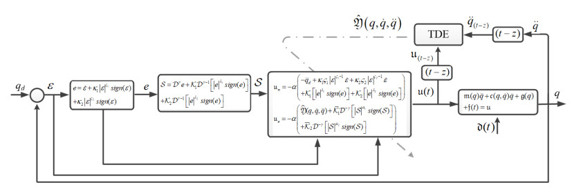
This paper presents a scheme of time-delay estimation (TDE) for unknown nonlinear robotic systems with uncertainty and external disturbances that utilizes fractional-order fixed-time sliding mode control (TDEFxFSMC). First, a detailed explanation and design concept of fractional-order fixed-time sliding mode control (FxFSMC) are provided. High performance tracking positions, non-chatter control inputs, and nonsingular fixed-time control are all realized with the FxSMC method. The proposed approach performs better and obtains superior performance when FxSMC is paired with fractional-order control. Furthermore, a TDE scheme is included in the suggested strategy to estimate the unknown nonlinear dynamics. Afterward, the suggested system's capacity to reach stability in fixed time is determined by using Lyapunov analyses. By showing the outcomes of the proposed technique applied to nonlinear robot dynamics, the efficacy of the recommended method is assessed, illustrated, and compared with the existing control scheme.
- time delay estimation,
- fractional-order control,
- fixed-time sliding mode control,
- nonlinear robotic system
Citation: Saim Ahmed, Ahmad Taher Azar, Ibraheem Kasim Ibraheem. Model-free scheme using time delay estimation with fixed-time FSMC for the nonlinear robot dynamics[J]. AIMS Mathematics, 2024, 9(4): 9989-10009. doi: 10.3934/math.2024489

Related Papers:

Abstract

This paper presents a scheme of time-delay estimation (TDE) for unknown nonlinear robotic systems with uncertainty and external disturbances that utilizes fractional-order fixed-time sliding mode control (TDEFxFSMC). First, a detailed explanation and design concept of fractional-order fixed-time sliding mode control (FxFSMC) are provided. High performance tracking positions, non-chatter control inputs, and nonsingular fixed-time control are all realized with the FxSMC method. The proposed approach performs better and obtains superior performance when FxSMC is paired with fractional-order control. Furthermore, a TDE scheme is included in the suggested strategy to estimate the unknown nonlinear dynamics. Afterward, the suggested system's capacity to reach stability in fixed time is determined by using Lyapunov analyses. By showing the outcomes of the proposed technique applied to nonlinear robot dynamics, the efficacy of the recommended method is assessed, illustrated, and compared with the existing control scheme.

References

[1]	A. T. Azar, Q. Zhu, A. Khamis, D. Zhao, Control design approaches for parallel robot manipulators: a review, Int. J. Model. Identif. Control, 28 (2017), 199–211. https://doi.org/10.1504/IJMIC.2017.086563 doi: 10.1504/IJMIC.2017.086563
[2]	K. K. Ayten, M. H. Çiplak, A. Dumlu, Implementation a fractional-order adaptive model-based PID-type sliding mode speed control for wheeled mobile robot, Proceedings of the Institution of Mechanical Engineers, Part Ⅰ: Journal of Systems and Control Engineering, 233 (2019), 1067–1084. https://doi.org/10.1177/0959651819847395 doi: 10.1177/0959651819847395
[3]	M. S. Zanjani, S. Mobayen, Event-triggered global sliding mode controller design for anti-sway control of offshore container cranes, Ocean Eng., 268 (2023), 113472. https://doi.org/10.1016/j.oceaneng.2022.113472 doi: 10.1016/j.oceaneng.2022.113472
[4]	M. Bakouri, A. Alqarni, S. Alanazi, A. Alassaf, I. AlMohimeed, M. A. Aboamer, et al., Robust dynamic control algorithm for uncertain powered wheelchairs based on sliding neural network approach, AIMS Math., 8 (2023), 26821–26839. https://doi.org/10.3934/math.20231373 doi: 10.3934/math.20231373
[5]	A. Almasoud, Jamming-aware optimization for UAV trajectory design and internet of things devices clustering, Complex Intell. Syst., 9 (2023), 4571–4590. https://doi.org/10.1007/s40747-023-00970-3 doi: 10.1007/s40747-023-00970-3
[6]	S. Ahmed, A. T. Azar, Adaptive fractional tracking control of robotic manipulator using fixed-time method, Complex Intell. Syst., 9 (2023), 369–382. https://doi.org/10.1007/s40747-023-01164-7 doi: 10.1007/s40747-023-01164-7
[7]	S. Ahmed, A. T. Azar, M. Tounsi, I. K. Ibraheem, Adaptive control design for Euler-Lagrange systems using fixed-time fractional integral sliding mode scheme, Fractal Fract., 7 (2023), 712. https://doi.org/10.3390/fractalfract7100712 doi: 10.3390/fractalfract7100712
[8]	S. J. Gambhire, D. R. Kishore, P. S. Londhe, S. N. Pawar, Review of sliding mode based control techniques for control system applications, Int. J. Dyn. Control, 9 (2021), 363–378. https://doi.org/10.1007/s40435-020-00638-7 doi: 10.1007/s40435-020-00638-7
[9]	H. Yin, B. Meng, Z. Wang, Disturbance observer-based adaptive sliding mode synchronization control for uncertain chaotic systems, AIMS Math., 8 (2023), 23655–23673. https://doi.org/10.3934/math.20231203 doi: 10.3934/math.20231203
[10]	D. Zhao, S. Li, F. Gao, A new terminal sliding mode control for robotic manipulators, Int. J. Control, 82 (2009), 1804–1813. https://doi.org/10.1080/00207170902769928 doi: 10.1080/00207170902769928
[11]	Y. Feng, X. Yu, Z. Man, Non-singular terminal sliding mode control of rigid manipulators, Automatica, 38 (2002), 2159–2167. https://doi.org/10.1016/S0005-1098(02)00147-4 doi: 10.1016/S0005-1098(02)00147-4
[12]	L. Yang, J. Yang, Nonsingular fast terminal sliding-mode control for nonlinear dynamical systems, Int. J. Robust Nonlinear Control, 21 (2011), 1865–1879. https://doi.org/10.1002/rnc.1666 doi: 10.1002/rnc.1666
[13]	C. Ton, C. Petersen, Continuous fixed-time sliding mode control for spacecraft with flexible appendages, IFAC-PapersOnLine, 51 (2018), 1–5. https://doi.org/10.1016/j.ifacol.2018.07.079 doi: 10.1016/j.ifacol.2018.07.079
[14]	H. Khan, S. Ahmed, J. Alzabut, A. T. Azar, J. F. Gómez-Aguilar, Nonlinear variable order system of multi-point boundary conditions with adaptive finite-time fractional-order sliding mode control, Int. J. Dyn. Control, 2024, 1–17. https://doi.org/10.1007/s40435-023-01369-1
[15]	Y. Su, C. Zheng, P. Mercorelli, Robust approximate fixed-time tracking control for uncertain robot manipulators, Mech. Syst. Signal Pr., 135 (2020), 106379. https://doi.org/10.1016/j.ymssp.2019.106379 doi: 10.1016/j.ymssp.2019.106379
[16]	S. Ahmed, A. T. Azar, I. K. Ibraheem, Nonlinear system controlled using novel adaptive fixed-time SMC, AIMS Math., 9 (2024), 7895–7916. https://doi.org/10.3934/math.2024384 doi: 10.3934/math.2024384
[17]	Z. Zhu, Z. Duan, H. Qin, Y. Xue, Adaptive neural network fixed-time sliding mode control for trajectory tracking of underwater vehicle, Ocean Eng., 287 (2023), 115864. https://doi.org/10.1016/j.oceaneng.2023.115864 doi: 10.1016/j.oceaneng.2023.115864
[18]	Q. D. Nguyen, D. D. Vu, S. C. Huang, V. N. Giap, Fixed-time supper twisting disturbance observer and sliding mode control for a secure communication of fractional-order chaotic systems, J. Vib. Control, 2023. https://doi.org/10.1177/10775463231180947
[19]	I. Podlubny, Fractional differential equations: an introduction to fractional derivatives, fractional differential equations, to methods of their solution and some of their applications, Elsevier, 1998.
[20]	A. Ali, K. Shah, T. Abdeljawad, H. Khan, A. Khan, Study of fractional order pantograph type impulsive antiperiodic boundary value problem, Adv. Differ. Equ., 2020 (2020), 572. https://doi.org/10.1186/s13662-020-03032-x doi: 10.1186/s13662-020-03032-x
[21]	S. Ahmad, A. Ullah, Q. M. Al-Mdallal, H. Khan, K. Shah, A. Khan, Fractional order mathematical modeling of COVID-19 transmission, Chaos Soliton. Fract., 139 (2020), 110256. https://doi.org/10.1016/j.chaos.2020.110256 doi: 10.1016/j.chaos.2020.110256
[22]	K. Shah, Z. A. Khan, A. Ali, R. Amin, H. Khan, A. Khan, Haar wavelet collocation approach for the solution of fractional order COVID-19 model using Caputo derivative, Alexandria Eng. J., 59 (2020), 3221–3231. https://doi.org/10.1016/j.aej.2020.08.028 doi: 10.1016/j.aej.2020.08.028
[23]	A. I. Ahmed, M. S. Al-Sharif, M. S. Salim, T. A. Al-Ahmary, Numerical solution of fractional variational and optimal control problems via fractional-order Chelyshkov functions, AIMS Math., 7 (2022), 17418–17443. https://doi.org/10.3934/math.2022960 doi: 10.3934/math.2022960
[24]	R. Ayad, W. Nouibat, M. Zareb, Y. B. Sebanne, Full control of quadrotor aerial robot using fractional-order FOPID, Iran. J. Sci. Technol. Trans. Electr. Eng., 43 (2019), 349–360. https://doi.org/10.1007/s40998-018-0155-4 doi: 10.1007/s40998-018-0155-4
[25]	H. Khan, S. Ahmed, J. Alzabut, A. T. Azar, A generalized coupled system of fractional differential equations with application to finite time sliding mode control for Leukemia therapy, Chaos Soliton. Fract., 174 (2023), 113901. https://doi.org/10.1016/j.chaos.2023.113901 doi: 10.1016/j.chaos.2023.113901
[26]	T. T. Nguyen, Fractional-order sliding mode controller for the two-link robot arm, Int. J. Electr. Comput. Eng., 10 (2020), 5579–5585. https://doi.org/10.11591/ijece.v10i6.pp5579-5585 doi: 10.11591/ijece.v10i6.pp5579-5585
[27]	S. Huang, L. Xiong, J. Wang, P. Li, Z. Wang, M. Ma, Fixed-time fractional-order sliding mode controller for multimachine power systems, IEEE Trans. Power Syst., 36 (2020), 2866–2876. https://doi.org/10.1109/TPWRS.2020.3043891 doi: 10.1109/TPWRS.2020.3043891
[28]	B. D. H. Phuc, V. D. Phung, S. S. You, T. D. Do, Fractional-order sliding mode control synthesis of supercavitating underwater vehicles, J. Vib. Control, 26 (2020), 1909–1919. https://doi.org/10.1177/1077546320908412 doi: 10.1177/1077546320908412
[29]	X. Zhang, F. Wu, M. Liu, X. Chen, Fractional-order robust fixed-time sliding mode control for deployment of tethered satellite, Acta Astronaut., 209 (2023), 172–178. https://doi.org/10.1016/j.actaastro.2023.04.041 doi: 10.1016/j.actaastro.2023.04.041
[30]	T. C. Lin, T. Y. Lee, V. E. Balas, Adaptive fuzzy sliding mode control for synchronization of uncertain fractional order chaotic systems, Chaos Soliton. Fract., 44 (2011), 791–801. https://doi.org/10.1016/j.chaos.2011.04.005 doi: 10.1016/j.chaos.2011.04.005
[31]	S. Huang, J. Wang, C. Huang, L. Zhou, L. Xiong, J. Liu, et al., A fixed-time fractional-order sliding mode control strategy for power quality enhancement of PMSG wind turbine, Int. J. Electr. Power Energy Syst., 134 (2022), 107354. https://doi.org/10.1016/j.ijepes.2021.107354 doi: 10.1016/j.ijepes.2021.107354
[32]	S. Han, H. Wang, Y. Tian, N. Christov, Time-delay estimation based computed torque control with robust adaptive RBF neural network compensator for a rehabilitation exoskeleton, ISA Trans., 97 (2020), 171–181. https://doi.org/10.1016/j.isatra.2019.07.030 doi: 10.1016/j.isatra.2019.07.030
[33]	A. T. Azar, H. H. Ammar, M. Y. Beb, S. R. Garces, A. Boubakari, Optimal design of PID controller for 2-DOF drawing robot using bat-inspired algorithm, In: A. Hassanien, K. Shaalan, M. Tolba, Proceedings of the International Conference on Advanced Intelligent Systems and Informatics 2019, Springer, 1058 (2019), 175–186. https://doi.org/10.1007/978-3-030-31129-2_17
[34]	M. Van, S. S. Ge, H. Ren, Finite time fault tolerant control for robot manipulators using time delay estimation and continuous nonsingular fast terminal sliding mode control, IEEE Trans. Cybernetics, 47 (2016), 1681–1693. https://doi.org/10.1109/TCYB.2016.2555307 doi: 10.1109/TCYB.2016.2555307
[35]	K. Y. Toumi, O. Ito, A time delay controller for systems with unknown dynamics, J. Dyn. Sys., Meas., Control, 112 (1990), 133–142. https://doi.org/10.1115/1.2894130 doi: 10.1115/1.2894130
[36]	T. C. Hsia, L. S. Gao, Robot manipulator control using decentralized linear time-invariant time-delayed joint controllers, Proceedings., IEEE International Conference on Robotics and Automation, IEEE, 1990, 2070–2075. https://doi.org/10.1109/ROBOT.1990.126310
[37]	S. Ahmed, I. Ghous, F. Mumtaz, TDE based model-free control for rigid robotic manipulators under nonlinear friction, Sci. Iran., 2022. https://doi.org/10.24200/sci.2022.57252.5141
[38]	Y. Wu, H. Fang, T. Xu, F. Wan, Adaptive neural fixed-time sliding mode control of uncertain robotic manipulators with input saturation and prescribed constraints, Neural Process. Lett., 54 (2022), 3829–3849. https://doi.org/10.1007/s11063-022-10788-8 doi: 10.1007/s11063-022-10788-8
[39]	A. Polyakov, Fixed-time stabilization via second order sliding mode control, IFAC Proc. Vol., 45 (2012), 254–258. https://doi.org/10.3182/20120606-3-NL-3011.00109 doi: 10.3182/20120606-3-NL-3011.00109
[40]	J. Zhai, Z. Li, Fast-exponential sliding mode control of robotic manipulator with super-twisting method, IEEE Trans. Circuits Syst. II, 69 (2021), 489–493. https://doi.org/10.1109/TCSII.2021.3081147 doi: 10.1109/TCSII.2021.3081147
[41]	S. Ahmed, A. T. Azar, M. Tounsi, Adaptive fault tolerant non-singular sliding mode control for robotic manipulators based on fixed-time control law, Actuators, 11 (2022), 353. https://doi.org/10.3390/act11120353 doi: 10.3390/act11120353
[42]	S. Ahmed, H. Wang, Y. Tian, Fault tolerant control using fractional-order terminal sliding mode control for robotic manipulators, Stud. Inform. Control, 27 (2018), 55–64. https://doi.org/10.24846/v27i1y201806 doi: 10.24846/v27i1y201806

Reader Comments

Your name:*

Email:*
© 2024 the Author(s), licensee AIMS Press. This is an open access article distributed under the terms of the Creative Commons Attribution License (http://creativecommons.org/licenses/by/4.0)