On the stability analysis of numerical schemes for solving non-linear polynomials arises in engineering problems

Mudassir Shams; Nasreen Kausar; Serkan Araci; Liang Kong; Mudassir Shams; Nasreen Kausar; Serkan Araci; Liang Kong

doi:10.3934/math.2024433

AIMS Mathematics

2024, Volume 9, Issue 4: 8885-8903. doi: 10.3934/math.2024433

Previous Article Next Article

Research article Special Issues

On the stability analysis of numerical schemes for solving non-linear polynomials arises in engineering problems

1.
Faculty of Engineering, Free University of Bozen-Bolzano (BZ), 39100, Italy
2.
Department of Mathematics and Statistics, Riphah International University I-14, Islamabad 44000, Pakistan
3.
Department of Mathematics, Faculty of Arts and Science, Yildiz Technical University, Esenler 34220, Istanbul, Türkiye
4.
Department of Basic Sciences, Faculty of Engineering, Hasan Kalyoncu University, TR-27010 Gaziantep, Türkiye
5.
Department of Mathematical Sciences and Philosophy, University of Illinois Springfield, USA

Received: 24 December 2023 Revised: 13 February 2024 Accepted: 19 February 2024 Published: 04 March 2024
MSC : 65H04, 65H05, 65Y05, 65M12

This study shows the link between computer science and applied mathematics. It conducts a dynamics investigation of new root solvers using computer tools and develops a new family of single-step simple root-finding methods. The convergence order of the proposed family of iterative methods is two, according to the convergence analysis carried out using symbolic computation in the computer algebra system CAS-Maple 18. Without further evaluations of a given nonlinear function and its derivatives, a very rapid convergence rate is achieved, demonstrating the remarkable computing efficiency of the novel technique. To determine the simple roots of nonlinear equations, this paper discusses the dynamic analysis of one-parameter families using symbolic computation, computer animation, and multi-precision arithmetic. To choose the best parametric value used in iterative schemes, it implements the parametric and dynamical plane technique using CAS-MATLAB$ ^{@}R2011b. $ The dynamic evaluation of the methods is also presented utilizing basins of attraction to analyze their convergence behavior. Aside from visualizing iterative processes, this method illustrates not only iterative processes but also gives useful information regarding the convergence of the numerical scheme based on initial guessed values. Some nonlinear problems that arise in science and engineering are used to demonstrate the performance and efficiency of the newly developed method compared to the existing method in the literature.
- complex dynamics,
- parametric plane,
- stability region,
- cpu time,
- engineering application
Citation: Mudassir Shams, Nasreen Kausar, Serkan Araci, Liang Kong. On the stability analysis of numerical schemes for solving non-linear polynomials arises in engineering problems[J]. AIMS Mathematics, 2024, 9(4): 8885-8903. doi: 10.3934/math.2024433

Related Papers:

Abstract

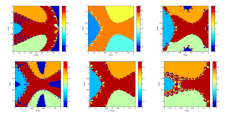
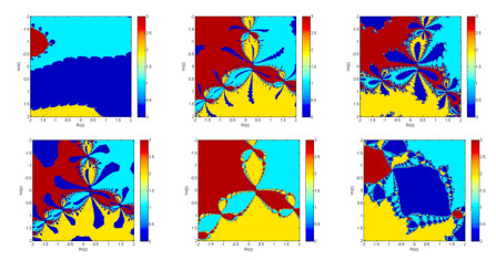
This study shows the link between computer science and applied mathematics. It conducts a dynamics investigation of new root solvers using computer tools and develops a new family of single-step simple root-finding methods. The convergence order of the proposed family of iterative methods is two, according to the convergence analysis carried out using symbolic computation in the computer algebra system CAS-Maple 18. Without further evaluations of a given nonlinear function and its derivatives, a very rapid convergence rate is achieved, demonstrating the remarkable computing efficiency of the novel technique. To determine the simple roots of nonlinear equations, this paper discusses the dynamic analysis of one-parameter families using symbolic computation, computer animation, and multi-precision arithmetic. To choose the best parametric value used in iterative schemes, it implements the parametric and dynamical plane technique using CAS-MATLAB$ ^{@}R2011b. $ The dynamic evaluation of the methods is also presented utilizing basins of attraction to analyze their convergence behavior. Aside from visualizing iterative processes, this method illustrates not only iterative processes but also gives useful information regarding the convergence of the numerical scheme based on initial guessed values. Some nonlinear problems that arise in science and engineering are used to demonstrate the performance and efficiency of the newly developed method compared to the existing method in the literature.

References

[1]	M. Cosnard, P. Fraigniaud, Finding the roots of a polynomial on an MIMD multicomputer, Parall. Comput., 15 (1990), 75–85. https://doi.org/10.1016/0167-8191(90)90032-5 doi: 10.1016/0167-8191(90)90032-5
[2]	X. Lü, H. Hui, F. Liu, Y. Bai, Stability and optimal control strategies for a novel epidemic model of COVID-19, Nonlinear Dyn., 106 (2021), 1491–1507. https://doi.org/10.1007/s11071-021-06524-x doi: 10.1007/s11071-021-06524-x
[3]	A. Naseem, M. Rehman, T. Abdeljawad, Computational methods for non-linear equations with some real-world applications and their graphical analysis, Intell. Autom. Soft Comput., 30 (2021), 805–819. http://dx.doi.org/10.32604/iasc.2021.019164 doi: 10.32604/iasc.2021.019164
[4]	B. Liu, X. E. Zhang, B. Wang, X. Lü, Rogue waves based on the coupled nonlinear Schrödinger option pricing model with external potential, Mod. Phys. Lett. B, 36 (2022), 2250057. https://doi.org/10.1142/S0217984922500579 doi: 10.1142/S0217984922500579
[5]	O. Aberth, Iteration methods for finding all zeros of a polynomial simultaneously, Math. Comput., 27 (1973), 339–344.
[6]	S. M. Kang, A. Rafiq, S. Ahmad, Y. C. Kwun, New iterative method with higher-order convergence for scalar equations, Int. J. Math. Anal., 10 (2016), 339–356. http://dx.doi.org/10.12988/ijma.2016.612 doi: 10.12988/ijma.2016.612
[7]	O. S. Solaiman, I. Hashim, Optimal eighth-order solver for nonlinear equations with applications in chemical engineering, Intell. Autom. Soft Comput., 27 (2021), 379–390. http://dx.doi.org/10.32604/iasc.2021.015285 doi: 10.32604/iasc.2021.015285
[8]	H. T. Kung, J. F. Traub, Optimal order of one-point and multipoint iteration, J. ACM, 21 (1974), 643–651. https://doi.org/10.1145/321850.321860 doi: 10.1145/321850.321860
[9]	M. Shams, N. Rafiq, N. Kausar, P. Agarwal, C. Park, S. Momani, Efficient iterative methods for finding simultaneously all the multiple roots of polynomial equation, Adv. Differ. Equ., 2021 (2021), 495. https://doi.org/10.1186/s13662-021-03649-6 doi: 10.1186/s13662-021-03649-6
[10]	S. A. Sariman, I. Hashim, New optimal Newton-Householder methods for solving nonlinear equations and their dynamics, Comput. Mater. Contin., 65 (2020), 69–85. http://dx.doi.org/10.32604/cmc.2020.010836 doi: 10.32604/cmc.2020.010836
[11]	M. A. Noor, K. I. Noor, W. A. Khan, F. Ahmad, On iterative methods for nonlinear equations, Appl. Math. Comput., 183 (2006), 128–133. http://dx.doi.org/10.1016/j.amc.2006.05.054 doi: 10.1016/j.amc.2006.05.054
[12]	O. Bazighifan, P. Kumam, Oscillation theorems for advanced differential equations with p-Laplacian like operators, Mathematics, 8 (2020), 821. https://doi.org/10.3390/math8050821 doi: 10.3390/math8050821
[13]	O. Moaaz, R. A. El-Nabulsi, O. Bazighifan, Oscillatory behavior of fourth-order differential equations with neutral delay, Symmetry, 12 (2020), 371. https://doi.org/10.3390/sym12030371 doi: 10.3390/sym12030371
[14]	O. Bazighifan, H. Alotaibi, A. A. A. Mousa, Neutral delay differential equations: Oscillation conditions for the solutions, Symmetry, 13 (2021), 101. https://doi.org/10.3390/sym13010101 doi: 10.3390/sym13010101
[15]	R. A. El-Nabulsi, O. Moaaz, O. Bazighifan, New results for oscillatory behavior of fourth-order differential equations, Symmetry, 12 (2020), 136. https://doi.org/10.3390/sym12010136 doi: 10.3390/sym12010136
[16]	O. Moaaz, D. Chalishajar, O. Bazighifan, Some qualitative behavior of solutions of general class of difference equations, Mathematics, 7 (2019), 585. https://doi.org/10.3390/math7070585 doi: 10.3390/math7070585
[17]	D. A. Knoll, E. K. David, Jacobian-free Newton-Krylova methods: A survey of approaches and applications, J. Comput. Phy., 193 (2004), 357–397. https://doi.org/10.1016/j.jcp.2003.08.010 doi: 10.1016/j.jcp.2003.08.010
[18]	J. F. Lemieux, B. Tremblay, J. Sedláček, P. Tupper, S. Thomas, D. Huard, et al., Improving the numerical convergence of viscous-plastic sea ice models with the Jacobian-free Newton-Krylova method, J. Comput. Phy., 229 (2010), 2840–2852. https://doi.org/10.1016/j.jcp.2009.12.011 doi: 10.1016/j.jcp.2009.12.011
[19]	X. Y. Wu, A new continuation Newton-like method and its deformation, Appl. Math. Comput., 112 (2000), 75–78. https://doi.org/10.1016/S0096-3003(99)00049-1 doi: 10.1016/S0096-3003(99)00049-1
[20]	U. K. Qureshi, Z. A. Kalhoro, A. A. Shaikh, A. R. Nangraj, Trapezoidal second order convergence method for solving nonlinear problems, USJICT, 2 (2018), 111–114.
[21]	J. H. He, Variational iteration method-some recent results and new interpretations, J. Comput. Appl. Math., 207 (2007), 3–17. https://doi.org/10.1016/j.cam.2006.07.009 doi: 10.1016/j.cam.2006.07.009
[22]	B. Saheya, G. Q. Chen, Y. K. Sui, C. Y. Wu, A new Newton-like method for solving nonlinear equations, SpringerPlus, 5 (2016), 1269. https://doi.org/10.1186/s40064-016-2909-7 doi: 10.1186/s40064-016-2909-7
[23]	S. Abbasbandy, Improving Newton-Raphson method for nonlinear equations by modified Adomian de composition method, Appl. Math. Comput., 145 (2003), 887–893. https://doi.org/10.1016/S0096-3003(03)00282-0 doi: 10.1016/S0096-3003(03)00282-0
[24]	G. M. Sandquist, Z. R. Wilde, Introduction to System Science with MATLAB, Hoboken: John Wiley and Sons, 2023.
[25]	A. Sohail, Genetic algorithms in the fields of artificial intelligence and data sciences, Ann. Data Sci., 10 (2023), 1007–1018. https://doi.org/10.1007/s40745-021-00354-9 doi: 10.1007/s40745-021-00354-9
[26]	A. Y. Özban, Some new variants of Newton's method, Appl. Math. Lett., 17 (2004), 677–682. https://doi.org/10.1016/S0893-9659(04)90104-8 doi: 10.1016/S0893-9659(04)90104-8
[27]	J. Kou, Y. Li, A family of new Newton-like method, Appl. Math. Comput., 192 (2007), 162–167. https://doi.org/10.1016/j.amc.2007.02.129 doi: 10.1016/j.amc.2007.02.129
[28]	F. I. Chicharro, A. Cordero, N. Garrido, J. R. Torregrosa, Generating root-finder iterative methods of second order convergence and stability, Axioms, 8 (2019), 55. https://doi.org/10.3390/axioms8020055 doi: 10.3390/axioms8020055
[29]	A. Cordero, J. R. Torregrosa, Variants of Newton's method using fifth order quadrature formulas, Appl. Math. Comput., 190 (2007), 686–698. https://doi.org/10.1016/j.amc.2007.01.062 doi: 10.1016/j.amc.2007.01.062
[30]	J. Gerlach, Accelerated convergence in Newton's method, SIAM Review, 36 (1994), 272–276. https://doi.org/10.1137/1036057 doi: 10.1137/1036057
[31]	I. Gościniak, K. Gdawiec, Visual analysis of dynamics behavior of an iterative method depending on selected parameters and modifications, Entropy, 1 (2020), 737. https://doi.org/10.3390/e22070734 doi: 10.3390/e22070734
[32]	S. A. Siddiqui, A. Ahmad, Implementation of Newton's algorithm using FORTRAN, SN Comput. Sci., 1 (2020), 348. https://doi.org/10.1007/s42979-020-00360-3 doi: 10.1007/s42979-020-00360-3
[33]	M. Shams, N. Rafiq, N. Kausar, N. A. Mir, A. Alalyani, Computer oriented numerical scheme for solving engineering problems, Comput. Syst. Sci. Eng., 42 (2022), 689–701. http://dx.doi.org/10.32604/csse.2022.022269 doi: 10.32604/csse.2022.022269
[34]	S. Amat, S. Busquier, S. Plaza, Chaotic dynamics of a third-order Newton-type method, J. Math. Anal. Appl., 336 (2010), 24–32. https://doi.org/10.1016/j.jmaa.2010.01.047 doi: 10.1016/j.jmaa.2010.01.047
[35]	P. Fatou, Sur les equations fonctionnelles, Bull. Soc. Mat. France, 47 (1919), 161–271.
[36]	J. F. Traub, Computational complexity of iterative processes, SIAM J. Comput., 1 (1972), 167–179. https://doi.org/10.1137/0201012 doi: 10.1137/0201012
[37]	S. Kumar, J. Bhagwan, L. Jäntschi, Numerical simulation of multiple roots of van der Waals and CSTR problems with a derivative-free technique, AIMS Math., 8 (2023), 14288–14299. http://dx.doi.org/10.3934/math.2023731 doi: 10.3934/math.2023731
[38]	G. Thangkhenpau, S. Panday, L. C. Bolunduţ, L. Jäntschi, Efficient families of multi-point iterative methods and their self-acceleration with memory for solving nonlinear equations, Symmetry, 15 (2023), 1546. https://doi.org/10.3390/sym15081546 doi: 10.3390/sym15081546
[39]	E. Sharma, S. Panday, S. K. Mittal, D. M. Joița, L. L. Pruteanu, L. Jäntschi, Derivative-free families of with-and without-memory iterative methods for solving nonlinear equations and their engineering applications, Mathematics, 11 (2023), 4512. https://doi.org/10.3390/math11214512 doi: 10.3390/math11214512
[40]	S. Kumar, J. R. Sharma, J. Bhagwan, L. Jäntschi, Numerical solution of nonlinear problems with multiple roots using derivative-free algorithms, Symmetry, 15 (2023), 1249. https://doi.org/10.3390/sym15061249 doi: 10.3390/sym15061249
[41]	R. L. Burden, J. D. Faires, Boundary-value problems for ordinary differential equations, In: Numerical Analysis, $9^th$ edition, Boston: Belmount Thomson Brooks/Cole Press, 2011.
[42]	V. K. Srivastav, S. Thota, M. Kumar, A new trigonometrical algorithm for computing real root of non-linear transcendental equations, Int. J. Appl. Comput. Math., 5 (2019), 44. https://doi.org/10.1007/s40819-019-0600-8 doi: 10.1007/s40819-019-0600-8
[43]	M. I. Argyros, I. K. Argyros, S. Regmi, S. George, Generalized three step numerical methods for solving equations in Banach spaces, Mathematics, 10 (2022), 2621. https://doi.org/10.3390/math10152621 doi: 10.3390/math10152621
[44]	T. Lei, R. M. Y. Li, H. Fu, Dynamics analysis and fractional-order approximate entropy of inventory management nonlinear systems, Math. Prob. Eng., 2021 (2021), 5516703. https://doi.org/10.1155/2021/5516703 doi: 10.1155/2021/5516703
[45]	W. Li, L. Weng, K. Zhao, S. Zhao, P. Zhang, Research on the evaluation of real estate inventory management in China, Land, 10 (2021), 1283. https://doi.org/10.3390/land10121283 doi: 10.3390/land10121283
[46]	H. Ran, Construction and optimization of inventory management system via cloud-edge collaborative computing in supply chain environment in the Internet of Things era, Plos One, 16 (2021), e0259284. https://doi.org/10.1371/journal.pone.0259284 doi: 10.1371/journal.pone.0259284

Reader Comments

Your name:*

Email:*
© 2024 the Author(s), licensee AIMS Press. This is an open access article distributed under the terms of the Creative Commons Attribution License (http://creativecommons.org/licenses/by/4.0)