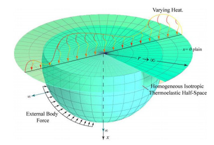
The thermal and mechanical properties of materials show differences depending on the temperature change, which necessitates consideration of the dependence of the properties of these materials on this change in the analysis of thermal stress and deformation of the material. As a result, in the present work, a mathematical framework for thermal conductivity was formulated to describe the behavior of non-simple elastic materials whose properties depend on temperature changes. This derived model includes generalized fractional differential operators with non-singular kernels and two-stage delay operators. The fractional derivative operators under consideration include both the Caputo-Fabrizio fractional derivative and the Atangana-Baleanu fractional derivative, in addition to the traditional fractional operator. Not only that, but the system of governing equations includes the concept of two temperatures. Based on the proposed model, the thermodynamic response of an unlimited, constrained thermoelastic medium subjected to laser pulses was considered. It was taken into account that the thermal elastic properties of the medium, such as the conductivity coefficient and specific heat, depend on the temperature. The governing equations of the problem were formulated and then solved using the Laplace transform method, followed by the numerical inverse. By presenting the numerical results in graphical form, a detailed analysis and discussion of the effects of fractional factors and the dependence of properties on temperature are presented. The results indicate that the fractional order coefficient, discrepancy index, and temperature-dependent properties significantly affect the behavior fluctuations of all physical domains under consideration.
Citation: Ibrahim-Elkhalil Ahmed, Ahmed E. Abouelregal, Doaa Atta, Meshari Alesemi. A fractional dual-phase-lag thermoelastic model for a solid half-space with changing thermophysical properties involving two-temperature and non-singular kernels[J]. AIMS Mathematics, 2024, 9(3): 6964-6992. doi: 10.3934/math.2024340
The thermal and mechanical properties of materials show differences depending on the temperature change, which necessitates consideration of the dependence of the properties of these materials on this change in the analysis of thermal stress and deformation of the material. As a result, in the present work, a mathematical framework for thermal conductivity was formulated to describe the behavior of non-simple elastic materials whose properties depend on temperature changes. This derived model includes generalized fractional differential operators with non-singular kernels and two-stage delay operators. The fractional derivative operators under consideration include both the Caputo-Fabrizio fractional derivative and the Atangana-Baleanu fractional derivative, in addition to the traditional fractional operator. Not only that, but the system of governing equations includes the concept of two temperatures. Based on the proposed model, the thermodynamic response of an unlimited, constrained thermoelastic medium subjected to laser pulses was considered. It was taken into account that the thermal elastic properties of the medium, such as the conductivity coefficient and specific heat, depend on the temperature. The governing equations of the problem were formulated and then solved using the Laplace transform method, followed by the numerical inverse. By presenting the numerical results in graphical form, a detailed analysis and discussion of the effects of fractional factors and the dependence of properties on temperature are presented. The results indicate that the fractional order coefficient, discrepancy index, and temperature-dependent properties significantly affect the behavior fluctuations of all physical domains under consideration.

| [1] |
H. Jordan, Transient heat conduction with variable thermophysical properties power-law temperature-dependent heat capacity and thermal conductivity, Therm. Sci., 27 (2023), 411–422. https://doi.org/10.2298/TSCI23S1411H doi: 10.2298/TSCI23S1411H

|
| [2] |
X. M. Wang, L. S. Zhang, C. Yang, N. Liu, W. L. Cheng, Estimation of temperature-dependent thermal conductivity and specific heat capacity for charring ablators, Int. J. Heat Mass Tran., 129 (2019), 894–902. https://doi.org/10.1016/j.ijheatmasstransfer.2018.10.014 doi: 10.1016/j.ijheatmasstransfer.2018.10.014
|
| [3] |
R. Tiwari, A. Singhal, A. Kumar, Effects of variable thermal properties on thermoelastic waves induced by sinusoidal heat source in half space medium, Mater. Today Proc., 62 (2022), 5099–5104. https://doi.org/10.1016/j.matpr.2022.02.442 doi: 10.1016/j.matpr.2022.02.442
|
| [4] |
A. E. Abouelregal, D. Atta, H. M. Sedighi, Vibrational behavior of thermoelastic rotating nanobeams with variable thermal properties based on memory-dependent derivative of heat conduction model, Arch. Appl. Mech., 93 (2023), 197–220. https://doi.org/10.1007/s00419-022-02110-8 doi: 10.1007/s00419-022-02110-8
|
| [5] | A. E. Abouelregal, H. Ahmad, S. W. Yao, H. Abu-Zinadah, Thermo-viscoelastic orthotropic constraint cylindrical cavity with variable thermal properties heated by laser pulse via the MGT thermoelasticity model, Open Phys., 19 (2021), 504–518. https://doi.org/10.1515/phys-2021-0034 |
| [6] |
A. E. Abouelregal, A comparative study of a thermoelastic problem for an infinite rigid cylinder with thermal properties using a new heat conduction model including fractional operators without non-singular kernels, Arch. Appl. Mech., 92 (2022), 3141–3161. https://doi.org/10.1007/s00419-022-02228-9 doi: 10.1007/s00419-022-02228-9
|
| [7] |
M. I. Khan, S. U. Khan, M. Jameel, Y. M. Chu, I. Tlili, S. Kadry, Significance of temperature-dependent viscosity and thermal conductivity of Walter's B nanoliquid when sinusodal wall and motile microorganisms density are significant, Surf. Interfaces, 22 (2021), 100849. https://doi.org/10.1016/j.surfin.2020.100849 doi: 10.1016/j.surfin.2020.100849
|
| [8] |
M. Sohail, U. Nazir, Y. M. Chu, H. Alrabaiah, W. Al-Kouz, P. Thounthong, Computational exploration for radiative flow of Sutterby nanofluid with variable temperature-dependent thermal conductivity and diffusion coefficient, Open Phys., 18 (2020), 1073–1083. https://doi.org/10.1515/phys-2020-0216 doi: 10.1515/phys-2020-0216
|
| [9] |
M. Ibrahim, T. Saeed, Y. M. Chu, H. M. Ali, G. Cheraghian, R. Kalbasi, Comprehensive study concerned graphene nano-sheets dispersed in ethylene glycol: Experimental study and theoretical prediction of thermal conductivity, Powder Technol., 386 (2021), 51–59. https://doi.org/10.1016/j.powtec.2021.03.028 doi: 10.1016/j.powtec.2021.03.028
|
| [10] | Adnan, S. Z. A. Zaidi, U. Khan, N. Ahmed, S. T. Mohyud-Din, Y. M. Chu, et al., Impacts of freezing temperature based thermal conductivity on the heat transfer gradient in nanofluids: applications for a curved Riga surface, Molecules, 25 (2020), 2152. https://doi.org/10.3390/molecules25092152 |
| [11] |
D. Khan, G. Ali, A. Khan, I. Khan, Y. M. Chu, K. S. Nisar, A new idea of fractal-fractional derivative with power law kernel for free convection heat transfer in a channel flow between two static upright parallel plates, Comput. Mater. Con., 65 (2020), 1237–1251. https://doi.org/10.32604/cmc.2020.011492 doi: 10.32604/cmc.2020.011492
|
| [12] |
I. Abbas, A. Hobiny, M. Marin, Photo-thermal interactions in a semi-conductor material with cylindrical cavities and variable thermal conductivity, J. Taibah Univ. Sci., 14 (2020), 1369–1376. https://doi.org/10.1080/16583655.2020.1824465 doi: 10.1080/16583655.2020.1824465
|
| [13] |
M. Fekry, M. I. Othman, Plane waves in generalized magneto-thermo-viscoelastic medium with voids under the effect of initial stress and laser pulse heating, Struct. Eng. Mech., 73 (2020), 621–629. https://doi.org/10.12989/sem.2020.73.6.621 doi: 10.12989/sem.2020.73.6.621
|
| [14] |
S. Banik, M. Kanoria, Effects of three-phase-lag on two-temperature generalized thermoelasticity for infinite medium with spherical cavity, Appl. Math. Mech.-Engl. Ed., 33 (2012), 483–498. https://doi.org/10.1007/s10483-012-1565-8 doi: 10.1007/s10483-012-1565-8
|
| [15] |
A. E. Abouelregal, K. M. Khalil, F. A. Mohammed, M. E. Nasr, A. Zakaria, I.-E. Ahmed, A generalized heat conduction model of higher-order time derivatives and three-phase-lags for non-simple thermoelastic materials, Sci. Rep., 10 (2020), 13625. https://doi.org/10.1038/s41598-020-70388-1 doi: 10.1038/s41598-020-70388-1
|
| [16] |
H. W. Lord, Y. Shulman, Generalized dynamical theory of thermoelasticity, J. Mech. Phys. Solids, 15 (1967), 299–309. https://doi.org/10.1016/0022-5096(67)90024-5 doi: 10.1016/0022-5096(67)90024-5
|
| [17] | A. E. Green, K. A. Lindsay, Thermoelasticity, J. Elasticity, 2 (1972), 1–7. https://doi.org/10.1007/BF00045689 |
| [18] |
D. Y. Tzou, The generalized lagging response in small-scale and high-rate heating, Int. J. Heat Mass Tran., 38 (1995), 3231–3240. https://doi.org/10.1016/0017-9310(95)00052-B doi: 10.1016/0017-9310(95)00052-B
|
| [19] |
D. Y. Tzou, Experimental support for the lagging behavior in heat propagation, J. Thermophys. Heat Tr., 9 (1995), 686–693. https://doi.org/10.2514/3.725 doi: 10.2514/3.725
|
| [20] |
S. K. R. Choudhuri, On a thermoelastic three-phase-lag model, J. Therm. Stresses, 30 (2007), 231–238. https://doi.org/10.1080/01495730601130919 doi: 10.1080/01495730601130919
|
| [21] |
A. E. Green, P. M. Naghdi, A re-examination of the basic results of thermomechanics, Proc. R. Soc. Lond. A, 432 (1991), 171–194. https://doi.org/10.1098/rspa.1991.0012 doi: 10.1098/rspa.1991.0012
|
| [22] |
A. E. Green, P. M. Naghdi, On undamped heat waves in an elastic solid, J. Therm. Stresses, 15 (1992), 253–264. https://doi.org/10.1080/01495739208946136 doi: 10.1080/01495739208946136
|
| [23] |
A. E. Green, P. M. Naghdi, Thermoelasticity without energy dissipation, J. Elasticity, 31 (1993), 189–208. https://doi.org/10.1007/BF00044969 doi: 10.1007/BF00044969
|
| [24] |
S. S. Askar, A. E. Abouelregal, A. Foul, H. M. Sedighi, Pulsed excitation heating of semiconductor material and its thermomagnetic response on the basis of fourth-order MGT photothermal model, Acta Mech., 234 (2023), 4977–4995. https://doi.org/10.1007/s00707-023-03639-7 doi: 10.1007/s00707-023-03639-7
|
| [25] |
A. E. Abouelregal, H. M. Sedighi, S. F. Megahid, Photothermal-induced interactions in a semiconductor solid with a cylindrical gap due to laser pulse duration using a fractional MGT heat conduction model, Arch. Appl. Mech., 93 (2023), 2287–2305. https://doi.org/10.1007/s00419-023-02383-7 doi: 10.1007/s00419-023-02383-7
|
| [26] |
A. E. Abouelregal, M. E. Nasr, O. Moaaz, H. M. Sedighi, Thermo-magnetic interaction in a viscoelastic micropolar medium by considering a higher-order two-phase-delay thermoelastic model, Acta Mech., 234 (2023), 2519–2541. https://doi.org/10.1007/s00707-023-03513-6 doi: 10.1007/s00707-023-03513-6
|
| [27] |
A. E. Abouelregal, O. Moaaz, K. M. Khalil, M. Abouhawwash, M. E. Nasr, Micropolar thermoelastic plane waves in microscopic materials caused by Hall-current effects in a two-temperature heat conduction model with higher-order time derivatives, Arch. Appl. Mech., 93 (2023), 1901–1924. https://doi.org/10.1007/s00419-023-02362-y doi: 10.1007/s00419-023-02362-y
|
| [28] |
D. Atta, A. E. Abouelregal, H. M. Sedighi, R. A. Alharb, Thermodiffusion interactions in a homogeneous spherical shell based on the modified Moore-Gibson-Thompson theory with two time delays, Mech. Time-Depen. Mater., 2023 (2023), 1–22. https://doi.org/10.1007/s11043-023-09598-9 doi: 10.1007/s11043-023-09598-9
|
| [29] |
M. E. Gurtin, W. O. Williams, On the clausius-duhem inequality, Z. Angew. Math. Phys., 17 (1966), 626–633. https://doi.org/10.1007/B6F01597243 doi: 10.1007/B6F01597243
|
| [30] |
P. J. Chen, M. E. Gurtin, On a theory of heat conduction involving two temperatures, Z. Angew. Math. Phys., 19 (1968), 614–627 (1968). https://doi.org/10.1007/BF01594969 doi: 10.1007/BF01594969
|
| [31] |
P. J. Chen, W. O. Williams, A note on non-simple heat conduction, Z. Angew. Math. Phys., 19 (1968), 969–970. https://doi.org/10.1007/BF01602278 doi: 10.1007/BF01602278
|
| [32] |
P. J. Chen, M. E. Gurtin, W. O. Williams, On the thermodynamics of non-simple elastic materials with two temperatures, Z. Angew. Math. Phys., 20 (1969), 107–112. https://doi.org/10.1007/BF01591120 doi: 10.1007/BF01591120
|
| [33] | W. E. Warren, P. J. Chen, Wave propagation in the two temperature theory of thermoelasticity, Acta Mech. 16 (1973), 21–33. https://doi.org/10.1007/BF01177123 |
| [34] | R. Quintanilla, On existence, structural stability, convergence and spatial behavior in thermoelasticity with two temperatures, Acta Mech., 168 (2004), 61–73. https://doi.org/10.1007/s00707-004-0073-6 |
| [35] |
S. Mondal, S. H. Mallik, M. Kanoria, Fractional order two-temperature dual-phase-lag thermoelasticity with variable thermal conductivity, International Scholarly Research Notices, 2014 (2014), 646049. https://doi.org/10.1155/2014/646049 doi: 10.1155/2014/646049
|
| [36] | S. G. Samko, A. A. Kilbas, O. I. Marichev, Fractional integrals and derivatives: theory and applications, Yverdon: Gordon and Breach Science Publishers, 1993. |
| [37] | K. S. Miller, B. Ross, An introduction to the fractional calculus and fractional differential equations, New York: John Wiley and Sons, 1993. |
| [38] | K. B. Oldman, J. Spanier, The fractional calculus, San Diego: Academic Press, 1974. |
| [39] | I. Podlubny, Fractional differential equations: an introduction to fractional derivatives, fractional differential equations, to methods of their solution and some of their applications, San Diego: Academic Press, 1999. |
| [40] |
K. M. Saad, New fractional derivative with non-singular kernel for deriving Legendre spectral collocation method, Alex. Eng. J., 59 (2020), 1909–1917. https://doi.org/10.1016/j.aej.2019.11.017 doi: 10.1016/j.aej.2019.11.017
|
| [41] |
M. Caputo, M. Fabrizio, A new definition of fractional derivative without singular kernel, Progr. Fract. Differ. Appl., 1 (2015), 73–85. http://doi.org/10.12785/pfda/010201 doi: 10.12785/pfda/010201
|
| [42] |
A. Abdon, B. Dumitru, New fractional derivatives with nonlocal and non-singular kernel: theory and application to heat transfer model, Therm. Sci., 20 (2016), 763–769. https://doi.org/10.2298/TSCI160111018A doi: 10.2298/TSCI160111018A
|
| [43] |
K. Hattaf, A new generalized definition of fractional derivative with non-singular kernel, Computation, 8 (2020), 49. https://doi.org/10.3390/computation8020049 doi: 10.3390/computation8020049
|
| [44] |
B. Ghanbari, S. Kumar, R. Kumar, A study of behaviour for immune and tumor cells in immunogenetic tumour model with non-singular fractional derivative, Chaos Solition. Fract., 133 (2020), 109619. https://doi.org/10.1016/j.chaos.2020.109619 doi: 10.1016/j.chaos.2020.109619
|
| [45] |
M. Al-Refai, T. Abdeljawad, Analysis of the fractional diffusion equations with fractional derivative of non-singular kernel, Adv. Differ. Equ., 2017 (2017), 315. https://doi.org/10.1186/s13662-017-1356-2 doi: 10.1186/s13662-017-1356-2
|
| [46] |
B. Ghanbari, A. Atangana, Some new edge detecting techniques based on fractional derivatives with non-local and non-singular kernels, Adv. Differ. Equ., 22020 (2020), 435. https://doi.org/10.1186/s13662-020-02890-9 doi: 10.1186/s13662-020-02890-9
|
| [47] |
B. Ghanbari, A new model for investigating the transmission of infectious diseases in a prey‐predator system using a non-singular fractional derivative, Math. Method. Appl. Sci., 46 (2023), 8106–8125. https://doi.org/10.1002/mma.7412 doi: 10.1002/mma.7412
|
| [48] | V. J. Prajapati, R. Meher, A robust analytical approach to the generalized Burgers-Fisher equation with fractional derivatives including singular and non-singular kernels, J. Ocean Eng. Sci., (2022). https://doi.org/10.1016/j.joes.2022.06.035 |
| [49] |
I. Slimane, G. Nazir, J. J. Nieto, F. Yaqoob, Mathematical analysis of Hepatitis C Virus infection model in the framework of non-local and non-singular kernel fractional derivative, Int. J. Biomath., 16 (2023), 2250064. https://doi.org/10.1142/S1793524522500644 doi: 10.1142/S1793524522500644
|
| [50] |
D. Lesan, On the thermodynamics of non-simple elastic materials with two temperatures, Z. Angew. Math. Phys., 21 (1970), 583–591. https://doi.org/10.1007/BF01587687 doi: 10.1007/BF01587687
|
| [51] | M. A. Ezzat, A. S. El Karamany, Fractional order heat conduction law in magneto-thermoelasticity involving two temperatures, Z. Angew. Math. Phys., 62 (2011), 937–952. https://doi.org/10.1007/s00033-011-0126-3 |
| [52] | J. K. Chen, J. E. Beraun, Numerical study of ultrashort laser pulse interactions with metal films. Numer. Heat Tr. A-Appl., 40 (2001), 1–20. https://doi.org/10.1080/104077801300348842 |
| [53] |
G. Honig, U. Hirdes, A method for the numerical inversion of Laplace transforms, J. Comput. Appl. Math., 10 (1984), 113–132. https://doi.org/10.1016/0377-0427(84)90075-X doi: 10.1016/0377-0427(84)90075-X
|
| [54] |
A. E. Abouelregal, A comparative study of a thermoelastic problem for an infinite rigid cylinder with thermal properties using a new heat conduction model including fractional operators without non-singular kernels, Arch. Appl. Mech., 92 (2022), 3141–3161. https://doi.org/10.1007/s00419-022-02228-9 doi: 10.1007/s00419-022-02228-9
|
| [55] |
A. E. Abouelregal, Two-temperature thermoelastic model without energy dissipation including higher order time-derivatives and two phase-lags, Mater. Res. Express, 6 (2019), 116535. https://doi.org/10.1088/2053-1591/ab447f doi: 10.1088/2053-1591/ab447f
|
| [56] |
R. Kumar, R. Prasad, R. Kumar, Thermoelastic interactions on hyperbolic two-temperature generalized thermoelasticity in an infinite medium with a cylindrical cavity, Eur. J. Mech. A-Solids, 82 (2020), 104007. https://doi.org/10.1016/j.euromechsol.2020.104007 doi: 10.1016/j.euromechsol.2020.104007
|
| [57] |
S. Deswal, K. K. Kalkal, S. S. Sheoran, Axi-symmetric generalized thermoelastic diffusion problem with two-temperature and initial stress under fractional order heat conduction, Physica B, 496 (2016), 57–68. https://doi.org/10.1016/j.physb.2016.05.008 doi: 10.1016/j.physb.2016.05.008
|
| [58] |
R. Tiwari, R. Kumar, A. Kumar, Investigation of thermal excitation induced by laser pulses and thermal shock in the half space medium with variable thermal conductivity, Wave. Random Complex, 32 (2022), 2313–2331. https://doi.org/10.1080/17455030.2020.1851067 doi: 10.1080/17455030.2020.1851067
|
| [59] |
A. Zenkour, A. Abouelregal, Nonlocal thermoelastic semi-infinite medium with variable thermal conductivity due to a laser short-pulse, J. Comput. Appl. Mech., 50 (2019), 90–98. https://doi.org/10.22059/JCAMECH.2019.276608.366 doi: 10.22059/JCAMECH.2019.276608.366
|
| [60] |
C. H. Chiu, C. K. Chen, Application of the decomposition method to thermal stresses in isotropic circular fins with temperature-dependent thermal conductivity, Acta Mech., 157 (2002), 147–158. https://doi.org/10.1007/BF01182160 doi: 10.1007/BF01182160
|


Figures(9) / Tables(4)

Ibrahim-Elkhalil Ahmed, Ahmed E. Abouelregal, Doaa Atta, Meshari Alesemi. A fractional dual-phase-lag thermoelastic model for a solid half-space with changing thermophysical properties involving two-temperature and non-singular kernels[J]. AIMS Mathematics, 2024, 9(3): 6964-6992. doi: 10.3934/math.2024340


 DownLoad: