Analyzing the dynamics of fractional spatio-temporal $ \mathrm{SEIR} $ epidemic model

A. E. Matouk; Ismail Gad Ameen; Yasmeen Ahmed Gaber; A. E. Matouk; Ismail Gad Ameen; Yasmeen Ahmed Gaber

doi:10.3934/math.20241489

AIMS Mathematics

2024, Volume 9, Issue 11: 30838-30863. doi: 10.3934/math.20241489

Previous Article Next Article

Research article

Analyzing the dynamics of fractional spatio-temporal $ \mathrm{SEIR} $ epidemic model

1.
Department of Mathematics, College of Science Al-Zulfi, Majmaah University, Al-Majmaah 11952, Saudi Arabia
2.
College of Engineering, Majmaah University, Al-Majmaah 11952, Saudi Arabia
3.
Department of Mathematics, Faculty of Science, South Valley University, Qena 83523, Egypt

Received: 02 August 2024 Revised: 08 October 2024 Accepted: 23 October 2024 Published: 30 October 2024
MSC : 26A33, 65R10, 92B05, 93D20

In this work, we present a comprehensive analysis of the spatio-temporal $ \mathrm{SEIR} $ epidemic model of fractional order. The infection dynamics in the proposed fractional order model (FOM) are described by a system of partial differential equations (PDEs) within a time-fractional order and diffusion operator in one-dimensional space, considering that the total population is split into four compartments: Susceptible, exposed, infected, and recovered individuals denoted as $ \mathrm{S} $, $ \mathrm{E} $, $ \mathrm{I} $ and $ \mathrm{R} $, respectively. Our contributions commence by establishing the existence and uniqueness of positively bounded solutions for the proposed FOM. Moreover, we determined all equilibrium points (EPs) and investigated their local stability based on the basic reproduction number (BRN) $ \mathcal{R}_{0} $, which is calculated by the next-generation matrix (NGM) method. Additionally, we demonstrated global stability using an appropriate Lyapunov function with fractional LaSalle's invariance principle (LIP). Sensitivity analysis of the FOM parameters was discussed to identify the most critical parameters by which the volume of disease propagation can be measured. The theoretical findings were corroborated by numerical simulations of solutions that are displayed in 3D and 2D graphs. Graphical simulations highlight the effect of vaccination on infection severity. Changing the fractional order $ \alpha $ in the proposed FOM has an influence on the speed of convergence to the steady state as a result of the memory effect. Furthermore, vaccination emerges as an effective strategy for disease control.
- mathematical modeling,
- fractional order model,
- basic reproduction number,
- stability analysis,
- numerical simulation
Citation: A. E. Matouk, Ismail Gad Ameen, Yasmeen Ahmed Gaber. Analyzing the dynamics of fractional spatio-temporal $ \mathrm{SEIR} $ epidemic model[J]. AIMS Mathematics, 2024, 9(11): 30838-30863. doi: 10.3934/math.20241489

Related Papers:

Abstract

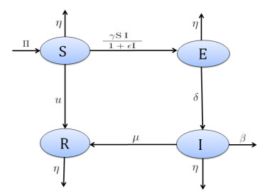
In this work, we present a comprehensive analysis of the spatio-temporal $ \mathrm{SEIR} $ epidemic model of fractional order. The infection dynamics in the proposed fractional order model (FOM) are described by a system of partial differential equations (PDEs) within a time-fractional order and diffusion operator in one-dimensional space, considering that the total population is split into four compartments: Susceptible, exposed, infected, and recovered individuals denoted as $ \mathrm{S} $, $ \mathrm{E} $, $ \mathrm{I} $ and $ \mathrm{R} $, respectively. Our contributions commence by establishing the existence and uniqueness of positively bounded solutions for the proposed FOM. Moreover, we determined all equilibrium points (EPs) and investigated their local stability based on the basic reproduction number (BRN) $ \mathcal{R}_{0} $, which is calculated by the next-generation matrix (NGM) method. Additionally, we demonstrated global stability using an appropriate Lyapunov function with fractional LaSalle's invariance principle (LIP). Sensitivity analysis of the FOM parameters was discussed to identify the most critical parameters by which the volume of disease propagation can be measured. The theoretical findings were corroborated by numerical simulations of solutions that are displayed in 3D and 2D graphs. Graphical simulations highlight the effect of vaccination on infection severity. Changing the fractional order $ \alpha $ in the proposed FOM has an influence on the speed of convergence to the steady state as a result of the memory effect. Furthermore, vaccination emerges as an effective strategy for disease control.

References

[1]	J. B. Mendel, J. T. Lee, D. Rosman, Current concepts imaging in COVID-19 and the challenges for low and middle income countries, J. Glob. Radiol., 6 (2020), 1106. https://doi.org/10.7191/jgr.2020.1106 doi: 10.7191/jgr.2020.1106
[2]	H. Fu, K. A. Gray, The key to maximizing the benefits of antimicrobial and self-cleaning coatings is to fully determine their risks, Curr. Opin. Chem. Eng., 34 (2021), 100761. https://doi.org/10.1016/j.coche.2021.100761 doi: 10.1016/j.coche.2021.100761
[3]	J. Dhar, A. Sharma, The role of the incubation period in a disease model, Appl. Math. E-Notes, 99 (2009), 146–153.
[4]	D. Bernoulli, Essai d'une nouvelle analyse de la mortalite causee par la petite verole et des avantages de l'inoculation pour la prevenir, Mem. Math. Phys. Acad. Roy. Sci., Paris., 1 (1760), 1–45.
[5]	N. Bacaër, A short history of mathematical population dynamics, London: Springer, 2011. https://doi.org/10.1007/978-0-85729-115-8_12
[6]	W. O. Kermack, A. G. McKendrick, A contribution to the mathematical theory of epidemics, Proc. R. Soc., Lond., Ser. A, 115 (1927), 700–721. https://doi.org/10.1098/rspa.1927.0118 doi: 10.1098/rspa.1927.0118
[7]	L. Acedo, G. González-Parra, A. J. Arenas, An exact global solution for the classical SIRS epidemic model, Nonlinear Anal. Real World Appl., 11 (2010), 1819–1825. https://doi.org/10.1016/j.nonrwa.2009.04.007 doi: 10.1016/j.nonrwa.2009.04.007
[8]	A. Omame, N. Sene, I. Nometa, C. I. Nwakanma, E. U. Nwafor, N. O. Iheonu, et al., Analysis of COVID-19 and comorbidity co-infection model with optimal control, Opt. Control Appl. Methods, 42 (2021), 568–590. https://doi.org/10.1002/oca.2748 doi: 10.1002/oca.2748
[9]	S. Paul, A. Mahata, U. Ghosh, B. Roy, Study of SEIR epidemic model and scenario analysis of COVID-19 pandemic, Ecol. Genet. Genom., 19 (2021), 100087. https://doi.org/10.1016/j.egg.2021.100087 doi: 10.1016/j.egg.2021.100087
[10]	M. Aakash, C. Gunasundari, Q. M. Al-Mdallal, Mathematical modeling and simulation of SEIR model for COVID-19 outbreak: A case study of Trivandrum, Front. Appl. Math. Stat., 9 (2023), 124897. https://doi.org/10.3389/fams.2023.1124897 doi: 10.3389/fams.2023.1124897
[11]	K. Hattaf, N. Yousfi, Global stability for reaction-diffusion equations in biology, Comput. Math. Appl., 66 (2013), 1488–1497. https://doi.org/10.1016/j.camwa.2013.08.023 doi: 10.1016/j.camwa.2013.08.023
[12]	J. Danane, K. Allali, L. M. Tine, V. Volpert, Nonlinear spatiotemporal viral infection model with CTL immunity: Mathematical analysis, Mathematics, 8 (2020), 52. https://doi.org/10.3390/math8010052 doi: 10.3390/math8010052
[13]	J. Zhou, Y. Ye, A. Arenas, S. Gómez, Yi Zhao, Pattern formation and bifurcation analysis of delay induced fractional-order epidemic spreading on networks, Chaos Soliton Fract., 174 (2023), 113805. https://doi.org/10.1016/j.chaos.2023.113805 doi: 10.1016/j.chaos.2023.113805
[14]	D. B. Meade, F. A. Milner, SIR epidemic models with directed diffusion, In: Mathematical aspects of human diseases applied mathematics monographs, 3 (1992), 1–10.
[15]	Y. Ye, J. Zhou, Yi Zhao, Pattern formation in reaction-diffusion information propagation model on multiplex simplicial complexes, Inform. Sci., 689 (2025), 121445. https://doi.org/10.1016/j.ins.2024.121445 doi: 10.1016/j.ins.2024.121445
[16]	L. Chang, S. Gao, Z. Wang, Optimal control of pattern formations for an SIR reaction-diffusion epidemic model, J. Theor. Biol., 536 (2022), 111003. https://doi.org/10.1016/j.jtbi.2022.111003 doi: 10.1016/j.jtbi.2022.111003
[17]	S. Chinviriyasit, W. Chinviriyasit, Numerical modelling of an SIR epidemic model with diffusion, Appl. Math. Comput., 216 (2010), 395–409. https://doi.org/10.1016/j.amc.2010.01.028 doi: 10.1016/j.amc.2010.01.028
[18]	K. Deng, Asymptotic behavior of an SIR reaction-diffusion model with a linear source, Discrete Contin. Dyn. Syst. Ser. B, 24 (2019), 5945–5957. https://doi.org/10.3934/dcdsb.2019114 doi: 10.3934/dcdsb.2019114
[19]	J. Danane, Z. Hammouch, K. Allali, S. Rashid, J. Singh, A fractional order model of coronavirus disease 2019 (COVID-19) with governmental action and individual reaction, Math. Methods Appl. Sci., 46 (2023), 8275–8288. https://doi.org/10.1002/mma.7759 doi: 10.1002/mma.7759
[20]	H. Qu, M. U. Rahman, S. Ahmad, M. B. Riazd, M. Ibrahim, T. Saeed, Investigation of fractional order bacteria dependent disease with the effects of different contact rates, Chaos Soliton Fract., 159 (2022), 112169. https://doi.org/10.1016/j.chaos.2022.112169 doi: 10.1016/j.chaos.2022.112169
[21]	L. Zhang, M. U. Rahman, S. Ahmad, M. B. Riaz, F. Jarad, Dynamics of fractional order delay model of coronavirus disease, AIMS Mathematics, 7 (2022), 4211–4232. https://doi.org/10.3934/math.2022234 doi: 10.3934/math.2022234
[22]	A. E. Matouk, Complex dynamics in susceptible-infected models for COVID-19 with multi-drug resistance, Chaos Soliton Fract., 140 (2020) 110257. https://doi.org/10.1016/j.chaos.2020.110257
[23]	R. Hilfer, Applications of fractional calculus in physics, World Scientifc, 2000. https://doi.org/10.1142/3779
[24]	I. Ameen, M. K. Elboree, R. O. Ahmed Tai, Traveling wave solutions to the nonlinear space-time fractional extended KdV equation via efficient analytical approaches, Alex Eng. J., 82 (2023), 468–483. https://doi.org/10.1016/j.aej.2023.10.022 doi: 10.1016/j.aej.2023.10.022
[25]	A. E. Matouk, I. Khan, Complex dynamics and control of a novel physical model using nonlocal fractional differential operator with singular kernel, J. Adv. Res., 24 (2020), 463–474. https://doi.org/10.1016/j.jare.2020.05.003 doi: 10.1016/j.jare.2020.05.003
[26]	A. Al-khedhairi, A. E. Matouk, I. Khan, Chaotic dynamics and chaos control for the fractional-order geomagnetic field model, Chaos Soliton Fract., 128 (2019) 390–401. https://doi.org/10.1016/j.chaos.2019.07.019
[27]	K. R. Cheneke, K. P. Rao, G. K. Edessa, Application of a new generalized fractional derivative and rank of control measures on cholera transmission dynamics, Int. J. Math. Math. Sci., 2021 (2021), 1–9. https://doi.org/10.1155/2021/2104051 doi: 10.1155/2021/2104051
[28]	R. P. Agarwal, D. Baleanu, J. J. Nieto, D. F. M. Torres, Y. Zhou, A survey on fuzzy fractional differential, and optimal control nonlocal evolution equations, J. Comput. Appl. Math., 339 (2018), 3–29. https://doi.org/10.1016/j.cam.2017.09.039 doi: 10.1016/j.cam.2017.09.039
[29]	A. E. Matouk, B. Lahcene, Chaotic dynamics in some fractional predator-prey models via a new Caputo operator based on the generalised Gamma function, Chaos Soliton Fract., 166 (2023), 112946. https://doi.org/10.1155/2020/5476842 doi: 10.1155/2020/5476842
[30]	W. W. Mohammed, E. S. Aly, A. E. Matouk, S. Albosaily, E. M. Elabbasy, An analytical study of the dynamic behavior of Lotka-Volterra based models of COVID-19, Results Phys., 26 (2021), 104432. https://doi.org/10.1016/j.camwa.08.039 doi: 10.1016/j.camwa.08.039
[31]	R. Almeida, D. Tavares, D. F. M. Torres, The variable-order fractional calculus of variations, Cham: Springer, 2019.
[32]	L. Debnath, Recent applications of fractional calculus to science and engineering, Int. J. Math. Math. Sci., 2003 (2003), 3413–3442. https://doi.org/10.1155/S0161171203301486 doi: 10.1155/S0161171203301486
[33]	A. Atangana, D. Baleanu, New fractional derivatives with nonlocal and nonsingular kernel: Theory and application to heat transfer model, Therm. Sci., 20 (2016). https://doi.org/10.48550/arXiv.1602.03408
[34]	W. Faridi, M. Fabrizio, A new defnition of fractional derivative without singular Kernel, Prog. Fract. Difer. Appl., 1 (2015), 73–85. https://doi.org/10.12785/pfda/010201 doi: 10.12785/pfda/010201
[35]	R. Khalil, M. A. Horani, A. Yousef, M. Sababheh, A new defnition of fractional derivative, Comput. Appl. Math., 264 (2014), 65–70. https://doi.org/10.1016/j.cam.2014.01.002 doi: 10.1016/j.cam.2014.01.002
[36]	M. Awadalla, J. Alahmadi, K. R. Cheneke, S. Qureshi, Fractional optimal control model and bifurcation analysis of human syncytial respiratory virus transmission dynamics, Fractal Fract., 8 (2024), 44. https://doi.org/10.3390/ractalfract8010044 doi: 10.3390/ractalfract8010044
[37]	K. Diethelm, A fractional calculus based model for the simulation of an outbreak of dengue fever, Nonlinear Dyn., 71 (2013), 613–619. https://doi.org/10.1007/s11071-012-0475-2 doi: 10.1007/s11071-012-0475-2
[38]	S. Rosa, D. F. M. Torres, Optimal control of a fractional order epidemic model with application to human respiratory syncytial virus infection, Chaos Soliton Fract., 117 (2018), 142–149. https://doi.org/10.1016/j.chaos.2018.10.021 doi: 10.1016/j.chaos.2018.10.021
[39]	A. B. Salati, M. Shamsi, D. F. M. Torres, Direct transcription methods based on fractional integral approximation formulas for solving nonlinear fractional optimal control problems, Commun. Nonlinear Sci. Numer. Simul., 67 (2019), 334–350. https://doi.org/10.1016/j.cnsns.2018.05.011 doi: 10.1016/j.cnsns.2018.05.011
[40]	S. Qureshi, A. Yusuf, Fractional derivatives applied to MSEIR problems: Comparative study with real world data, Eur. Phys. J. Plus., 134 (2019), 171. https://doi.org/10.1140/epjp/i2019-12661-7 doi: 10.1140/epjp/i2019-12661-7
[41]	Z. Ali, F. Rabiei, K. Shah, T. Khodadadi, Modeling and analysis of novel COVID-19 under fractal-fractional derivative with case study of Malaysia, Fractals, 29 (2021), 2150020. https://doi.org/10.1142/S0218348X21500201 doi: 10.1142/S0218348X21500201
[42]	H. Ali, I. Ameen, Y. A. Gaber, The effect of curative and preventive optimal control measures on a fractional order plant disease model, Math. Comput. Simul., 220 (2024), 496–515. https://doi.org/10.1016/j.matcom.2024.02.009 doi: 10.1016/j.matcom.2024.02.009
[43]	T. Kaisara, F. Nyabadza, Modelling Botswana's HIV/AIDS response and treatment policy changes: Insights from a cascade of mathematical models, Math. Biosci. Eng., 20 (2023), 1122–1147. https://doi.org/10.3934/mbe.2023052 doi: 10.3934/mbe.2023052
[44]	I. Sahu, S. R. Jena, SDIQR mathematical modelling for COVID-19 of Odisha associated with influx of migrants based on Laplace Adomian decomposition technique, Model. Earth Syst. Environ., 9 (2023), 4031–4040. https://doi.org/10.1007/s40808-023-01756-9 doi: 10.1007/s40808-023-01756-9
[45]	M. Li, J. Zu, The review of differential equation models of HBV infection dynamics, J. Virol. Methods., 266 (2019), 103–113. https://doi.org/10.1016/j.jviromet.2019.01.014 doi: 10.1016/j.jviromet.2019.01.014
[46]	V. Capasso, G. Serio, A generalization of the Kermack-Mckendrick deterministic epidemic model, Math. Biosci., 42 (1978), 42–43. https://doi.org/10.1016/0025-5564(78)90006-8 doi: 10.1016/0025-5564(78)90006-8
[47]	J. G. Wagner, Properties of the Michaelis-Menten equation and its integrated form which are useful in pharmacokinetics, J. Pharmacokinet. Biopharm., 1 (1973), 103–121. https://doi.org/10.1007/BF01059625 doi: 10.1007/BF01059625
[48]	E. A. Algehyne, R. Ud Din, On global dynamics of COVID-19 by using SQIR type model under non-linear saturated incidence rate, Alex. Eng. J., 60 (2021), 393–399. https://doi.org/10.1016/j.aej.2020.08.040 doi: 10.1016/j.aej.2020.08.040
[49]	Y. Yang, R. Xu, Mathematical analysis of a delayed HIV infection model with saturated CTL immune response and immune impairment, J. Appl. Math. Comput., 68 (2022), 2365–2380. https://doi.org/10.1007/s12190-021-01621-x doi: 10.1007/s12190-021-01621-x
[50]	K. Diethelm, The analysis of fractional differential equations, an application-oriented exposition using operators of Caputo type, Berlin: Springer, 2004.
[51]	S. A. Khuri, A Laplace decomposition algorithm applied to a class of nonlinear differential equations, J. Appl. Math., 1 (2001), 141–155. https://doi.org/10.1155/S1110757X01000183 doi: 10.1155/S1110757X01000183
[52]	R. Duduchava, The Green formula and layer potentials, Integr. Equ. Oper. Theory, 41 (2001), 127–178. https://doi.org/10.1007/BF01295303 doi: 10.1007/BF01295303
[53]	K. Hattaf, N. Yousf, Global stability for fractional diffusion equations in biological systems, Complexity, 2020 (2020), 5476842. https://doi.org/10.1155/2020/5476842 doi: 10.1155/2020/5476842
[54]	I. Petráš, Fractional-order nonlinear systems: Modeling, analysis and simulation, Springer, 2011.
[55]	J. P. C. Dos Santos, E. Monteiro, G. B. Vieira, Global stability of fractional SIR epidemic model, Proc. Ser. Braz. Soc. Appl. Comput. Math., 5 (2017), 1–7. https://doi.org/10.5540/03.2017.005.01.0019 doi: 10.5540/03.2017.005.01.0019
[56]	C. Vargas-De-León, Volterra-type Lyapunov functions for fractional-order epidemic systems, Commun. Nonlinear Sci. Numer. Simul., 24 (2015), 75–85. https://doi.org/10.1016/j.cnsns.2014.12.013 doi: 10.1016/j.cnsns.2014.12.013
[57]	N. Aguila-Camacho, M. A. Duarte-Mermoud, J. A. Gallegos, Lyapunov functions for fractional order systems, Commun. Nonlinear Sci. Numer. Simul., 19 (2014), 2951–2957. https://doi.org/10.1016/j.cnsns.2014.01.022 doi: 10.1016/j.cnsns.2014.01.022
[58]	M. M. El-Borai, Some probability densities and fundamental solutions of fractional evolution equations, Chaos Soliton Fract., 14 (2002), 433–440. https://doi.org/10.1016/S0960-0779(01)00208-9 doi: 10.1016/S0960-0779(01)00208-9
[59]	M. S. Tavazoei, M. Haeri, Chaotic attractors in incommensurate fractional order systems, Phys. D, 237 (2008), 2628–2637. https://doi.org/10.1016/j.physd.2008.03.037 doi: 10.1016/j.physd.2008.03.037
[60]	H. Caswell, Matrix population models, Wiley Online Library, 2006.
[61]	N. Chitnis, J. M. Hyman, J. M. Cushing, Determining important parameters in the spread of malaria through the sensitivity analysis of a mathematical model, Bull. Math. Biol., 70 (2008), 1272–1296. https://doi.org/10.1007/s11538-008-9299-0 doi: 10.1007/s11538-008-9299-0
[62]	K. W. Morton, D. F. Mayers, Numerical solution of partial differential equations: An introduction, Cambridge University Press, 2005.
[63]	C. Li, F. Zeng, Numerical methods for fractional calculus, Chapman & Hall/CRC, 2015.
[64]	Y. Lin, C. Xu, Finite diference/spectral approximations for the time-fractional difusion equation, J. Comput. Phys., 225 (2007), 1533–1552. https://doi.org/10.1016/j.jcp.2007.02.001 doi: 10.1016/j.jcp.2007.02.001
[65]	C. Bounkaicha, K. Allali, Modelling disease spread with spatio-temporal fractional derivative equations and saturated incidence rate, Model. Earth Syst. Environ., 10 (2024), 259–271. https://doi.org/10.1007/s40808-023-01773-8 doi: 10.1007/s40808-023-01773-8
[66]	C. M. Wachira, G. O. Lawi, L. O. Omondi, Travelling wave analysis of a diffusive COVID-19 model, J. Appl. Math., 2022 (2022), 6052274. https://doi.org/10.1155/2022/6052274 doi: 10.1155/2022/6052274

Reader Comments

Your name:*

Email:*
© 2024 the Author(s), licensee AIMS Press. This is an open access article distributed under the terms of the Creative Commons Attribution License (http://creativecommons.org/licenses/by/4.0)