A mathematical model for simulating the spread of infectious disease using the Caputo-Fabrizio fractional-order operator

Parveen Kumar; Sunil Kumar; Badr Saad T Alkahtani; Sara S Alzaid; Parveen Kumar; Sunil Kumar; Badr Saad T Alkahtani; Sara S Alzaid

doi:10.3934/math.20241490

AIMS Mathematics

2024, Volume 9, Issue 11: 30864-30897. doi: 10.3934/math.20241490

Previous Article Next Article

Research article Special Issues

A mathematical model for simulating the spread of infectious disease using the Caputo-Fabrizio fractional-order operator

1.
Department of Mathematics, National Institute of Technology, Jamshedpur, 831014, Jharkhand, India
2.
Department of Mathematics, College of Science, King Saud University, P.O. Box 2455, Riyadh 11451, Saudi Arabia

Received: 23 June 2024 Revised: 26 August 2024 Accepted: 09 September 2024 Published: 30 October 2024
MSC : 26A33, 34A08, 78A70, 93C10, 93C15

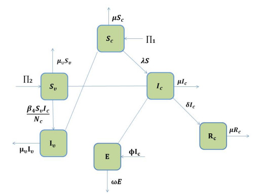
We examined intraspecific infectious rivalry in a dynamic contagious disease model. A non-linear dynamic model that considers multiple individual categories was used to study the transmission of infectious diseases. The combined effect of parameter sensitivities on the model was simulated using system sensitivities. To investigate the dynamic behavior and complexity of the model, the Caputo-Fabrizio (C-F) fractional derivative was utilized. The behavior of the proposed model around the parameters was examined using sensitivity analysis, and fractional solutions included more information than the classical model. Fixed point theory was used to analyze the existence and uniqueness of the solution. The Ulam-Hyers (U-H) criterion was used to examine the stability of the system. A numerical approach based on the C-F fractional operator was utilized to improve comprehension and treatment of the infectious disease model. A more precise and valuable technique for solving the infectious disease model was used in MATLAB numerical simulations to demonstrate. Time series and phase diagrams with different orders and parameters were generated. We aimed to expedite patient recovery while reducing the frequency of disease transmission in the community.
- infectious disease model,
- Caputo-Fabrizio derivative,
- snsitivity analysis,
- existence and uniqueness,
- numerical scheme
Citation: Parveen Kumar, Sunil Kumar, Badr Saad T Alkahtani, Sara S Alzaid. A mathematical model for simulating the spread of infectious disease using the Caputo-Fabrizio fractional-order operator[J]. AIMS Mathematics, 2024, 9(11): 30864-30897. doi: 10.3934/math.20241490

Related Papers:

Abstract

We examined intraspecific infectious rivalry in a dynamic contagious disease model. A non-linear dynamic model that considers multiple individual categories was used to study the transmission of infectious diseases. The combined effect of parameter sensitivities on the model was simulated using system sensitivities. To investigate the dynamic behavior and complexity of the model, the Caputo-Fabrizio (C-F) fractional derivative was utilized. The behavior of the proposed model around the parameters was examined using sensitivity analysis, and fractional solutions included more information than the classical model. Fixed point theory was used to analyze the existence and uniqueness of the solution. The Ulam-Hyers (U-H) criterion was used to examine the stability of the system. A numerical approach based on the C-F fractional operator was utilized to improve comprehension and treatment of the infectious disease model. A more precise and valuable technique for solving the infectious disease model was used in MATLAB numerical simulations to demonstrate. Time series and phase diagrams with different orders and parameters were generated. We aimed to expedite patient recovery while reducing the frequency of disease transmission in the community.

References

[1]	S. Kumar, A. Ahmadian, R. Kumar, D. Kumar, J. Singh, D. Baleanu, et al., An efficient numerical method for fractional SIR epidemic model of infectious disease by using Bernstein wavelets, Mathematics, 8 (2020), 1–22. https://doi.org/10.3390/math8040558 doi: 10.3390/math8040558
[2]	M. O. Oke, O. M. Ogunmiloro, C. T. Akinwumi, R. A. Raji, Mathematical modeling and stability analysis of a SIRV epidemic model with non-linear force of infection and treatment, Commun. Math. Appl., 10 (2019), 717–731. https://doi.org/10.26713/cma.v10i4.1172 doi: 10.26713/cma.v10i4.1172
[3]	W. F. Alfwzan, D. Baleanu, A. Raza, M. Rafiq, N. Ahmed, Dynamical analysis of a class of SEIR models through delayed strategies, AIP Adv., 13 (2023), 075115. https://doi.org/10.1063/5.0159942 doi: 10.1063/5.0159942
[4]	K. Umapathy, B. Palanivelu, R. Jayaraj, D. Baleanu, P. B. Dhandapani, On the decomposition and analysis of novel simultaneous SEIQR epidemic model, AIMS Math., 8 (2023), 5918–5933. https://doi.org/10.3934/math.2023298 doi: 10.3934/math.2023298
[5]	K. S. Mathur, P. Narayan, Dynamics of an SVEIRS epidemic model with vaccination and saturated incidence rate, Int. J. Appl. Comput. Math., 4 (2018), 118. https://doi.org/10.1007/s40819-018-0548-0 doi: 10.1007/s40819-018-0548-0
[6]	D. Kumar, J. Singh, M. Al Qurashi, D. Baleanu, A new fractional SIRS-SI malaria disease model with application of vaccines, antimalarial drugs, and spraying, Adv. Differ. Equ., 2019 (2019), 1–19. https://doi.org/10.1186/s13662-019-2199-9 doi: 10.1186/s13662-019-2199-9
[7]	J. Amador, The SEIQS stochastic epidemic model with external source of infection, Appl. Math. Model., 40 (2016), 8352–8365. https://doi.org/10.1016/j.apm.2016.04.023 doi: 10.1016/j.apm.2016.04.023
[8]	A. Atangana, D. Baleanu, Caputo-Fabrizio derivative applied to groundwater flow within confined aquifer, J. Eng. Mech., 143 (2017), D4016005. https://doi.org/10.1061/(ASCE)EM.1943-7889.0001091 doi: 10.1061/(ASCE)EM.1943-7889.0001091
[9]	D. Baleanu, A. Mousalou, S. Rezapour, On the existence of solutions for some infinite coefficient-symmetric Caputo-Fabrizio fractional integro-differential equations, Bound. Value Probl., 2017 (2017), 1–9. https://doi.org/10.1186/s13661-017-0867-9 doi: 10.1186/s13661-017-0867-9
[10]	P. Kumar, S. Kumar, B. S. T. Alkahtani, S. S. Alzaid, The complex dynamical behaviour of fractal-fractional forestry biomass system, Appl. Math. Sci. Eng., 32 (2024), 2375542. https://doi.org/10.1080/27690911.2024.2375542 doi: 10.1080/27690911.2024.2375542
[11]	P. Kumar, S. Kumar, B. S. T. Alkahtani, S. S. Alzaid, A robust numerical study on modified Lumpy skin disease model, AIMS Math., 9 (2024), 22941–22985. https://doi.org/10.3934/math.20241116 doi: 10.3934/math.20241116
[12]	P. Kumar, A. Kumar, S. Kumar, A study on fractional order infectious chronic wasting disease model in deers, Arab J. Basic Appl. Sci., 30 (2023), 601–625. https://doi.org/10.1080/25765299.2023.2270229 doi: 10.1080/25765299.2023.2270229
[13]	A. Atangana, D. Baleanu, New fractional derivatives with non-local and non-singular kernel: theory and application to heat transfer model, Thermal Sci., 20 (2016), 763–769. https://doi.org/10.2298/TSCI160111018A doi: 10.2298/TSCI160111018A
[14]	F. A. Rihan, Sensitivity analysis for dynamic systems with time-lags, J. Comput. Appl. Math., 151 (2003), 445–462. https://doi.org/10.1016/S0377-0427(02)00659-3 doi: 10.1016/S0377-0427(02)00659-3
[15]	I. A. Baba, F. A. Rihan, E. Hincal, A fractional order model that studies terrorism and corruption codynamics as epidemic disease, Chaos Solitons Fract., 169 (2023), 113292. https://doi.org/10.1016/j.chaos.2023.113292 doi: 10.1016/j.chaos.2023.113292
[16]	F. A. Rihan, U. Kandasamy, H. J. Alsakaji, N. Sottocornola, Dynamics of a fractional-order delayed model of COVID-19 with vaccination efficacy, Vaccines, 11 (2023), 1–26. https://doi.org/10.3390/vaccines11040758 doi: 10.3390/vaccines11040758
[17]	P. Kumar, A. Kumar, S. Kumar, D. Baleanu, A fractional order co-infection model between malaria and filariasis epidemic, Arab J. Basic Appl. Sci., 31 (2024), 132–153. https://doi.org/10.1080/25765299.2024.2314376 doi: 10.1080/25765299.2024.2314376
[18]	D. Baleanu, H. Mohammadi, S. Rezapour, A fractional differential equation model for the COVID-19 transmission by using the Caputo-Fabrizio derivative, Adv. Differ. Equ., 2020 (2020), 299. https://doi.org/10.1186/s13662-020-02762-2 doi: 10.1186/s13662-020-02762-2
[19]	S. Kumar, A. Kumar, M. Jleli, A numerical analysis for fractional model of the spread of pests in tea plants, Numer. Methods Partial Differ. Equ., 38 (2022), 540–565. https://doi.org/10.1002/num.22663 doi: 10.1002/num.22663
[20]	F. Evirgen, E. Uçar, S. Uçar, N. Özdemir, Modelling influenza a disease dynamics under {Caputo-Fabrizio} fractional derivative with distinct contact rates, Math. Model. Numer. Simul. Appl., 3 (2023), 58–73. https://doi.org/10.53391/mmnsa.1274004 doi: 10.53391/mmnsa.1274004
[21]	H. Joshi, M. Yavuz, Transition dynamics between a novel coinfection model of fractional-order for COVID-19 and tuberculosis via a treatment mechanism, Eur. Phys. J. Plus, 138 (2023), 468. https://doi.org/10.1140/epjp/s13360-023-04095-x doi: 10.1140/epjp/s13360-023-04095-x
[22]	F. Evirgen, E. Ucar, N. Özdemir, E. Altun, T. Abdeljawad, The impact of nonsingular memory on the mathematical model of Hepatitis C virus, Fractals, 31 (2023), 2340065. https://doi.org/10.1142/S0218348X23400650 doi: 10.1142/S0218348X23400650
[23]	M. ur Rahman, M. Arfan, D. Baleanu, Piecewise fractional analysis of the migration effect in plant-pathogen-herbivore interactions, Bull. Biomath., 1 (2023), 1–23. https://doi.org/10.59292/bulletinbiomath.2023001 doi: 10.59292/bulletinbiomath.2023001
[24]	H. Joshi, M. Yavuz, S. Townley, B. K. Jha, Stability analysis of a non-singular fractional-order covid-19 model with nonlinear incidence and treatment rate, Phys. Scr., 98 (2023), 045216. https://doi.org/10.1088/1402-4896/acbe7a doi: 10.1088/1402-4896/acbe7a
[25]	B. Fatima, M. Yavuz, M. ur Rahman, F. S. Al-Duais, Modeling the epidemic trend of middle eastern respiratory syndrome coronavirus with optimal control, Math. Biosci. Eng., 20 (2023), 11847–11874. https://doi.org/10.3934/mbe.2023527 doi: 10.3934/mbe.2023527
[26]	M. Toufik, A. Atangana, New numerical approximation of fractional derivative with non-local and non-singular kernel: application to chaotic models, Eur. Phys. J. Plus, 132 (2017), 1–16. https://doi.org/10.1140/epjp/i2017-11717-0 doi: 10.1140/epjp/i2017-11717-0
[27]	M. A. Khan, A. Atangana, Modeling the dynamics of novel coronavirus (2019-nCov) with fractional derivative, Alex. Eng. J., 59 (2020), 2379–2389. https://doi.org/10.1016/j.aej.2020.02.033 doi: 10.1016/j.aej.2020.02.033
[28]	S. M. Ulam, Problems in modern mathematics, Courier Corporation, 2004.
[29]	T. M. Rassias, On the stability of functional equations and a problem of Ulam, Acta Appl. Math., 62 (2000), 23–130. https://doi.org/10.1023/A:1006499223572 doi: 10.1023/A:1006499223572
[30]	S. Uçar, E. Uçar, N. Özdemir, Z. Hammouch, Mathematical analysis and numerical simulation for a smoking model with Atangana-Baleanu derivative, Chaos Solitons Fract., 118 (2019), 300–306. https://doi.org/10.1016/j.chaos.2018.12.003 doi: 10.1016/j.chaos.2018.12.003
[31]	J. Losada, J. J. Nieto, Properties of a new fractional derivative without singular kernel, Progr. Fract. Differ. Appl., 1 (2015), 87–92.
[32]	A. Atangana, I. Koca, Chaos in a simple nonlinear system with Atangana-Baleanu derivatives with fractional order, Chaos Solitons Fract., 89 (2016), 447–454. https://doi.org/10.1016/j.chaos.2016.02.012 doi: 10.1016/j.chaos.2016.02.012
[33]	S. Riaz, A. Ali, M. Munir, Sensitivity analysis of an infectious disease model under fuzzy impreciseness, Partial Differ. Equ. Appl. Math., 9 (2024), 100638. https://doi.org/10.1016/j.padiff.2024.100638 doi: 10.1016/j.padiff.2024.100638
[34]	I. Ahmed, A. Akgül, F. Jarad, P. Kumam, K. Nonlaopon, A Caputo-Fabrizio fractional-order cholera model and its sensitivity analysis, Math. Model. Numer. Simul. Appl., 3 (2023), 170–187. https://doi.org/10.53391/mmnsa.1293162 doi: 10.53391/mmnsa.1293162
[35]	N. Chitnis, J. M. Hyman, J. M. Cushing, Determining important parameters in the spread of malaria through the sensitivity analysis of a mathematical model, Bull. Math. Biol., 70 (2008), 1272–1296. https://doi.org/10.1007/s11538-008-9299-0 doi: 10.1007/s11538-008-9299-0
[36]	D. Baleanu, H. Mohammadi, S. Rezapour, A mathematical theoretical study of a particular system of Caputo-Fabrizio fractional differential equations for the Rubella disease model, Adv. Differ. Equ., 2020 (2020), 1–19. https://doi.org/10.1186/s13662-020-02614-z doi: 10.1186/s13662-020-02614-z
[37]	A. Chavada, N. Pathak, Transmission dynamics of breast cancer through Caputo Fabrizio fractional derivative operator with real data, Math. Model. Control, 4 (2024), 119–132. https://doi.org/10.3934/mmc.2024011 doi: 10.3934/mmc.2024011
[38]	D. H. Hyers, On the stability of the linear functional equation, Proc. Nat. Acad. Sci., 27 (1941), 222–224. https://doi.org/10.1073/pnas.27.4.222 doi: 10.1073/pnas.27.4.222
[39]	J. M. Rassias, Solution of a problem of Ulam, J. Approx. Theory, 57 (1989), 268–273. https://doi.org/10.1016/0021-9045(89)90041-5 doi: 10.1016/0021-9045(89)90041-5
[40]	S. M. Jung, Hyers-Ulam stability of linear differential equations of first order, Appl. Math. Lett., 17 (2004), 1135–1140. https://doi.org/10.1016/j.aml.2003.11.004 doi: 10.1016/j.aml.2003.11.004
[41]	S. M. Jung, Hyers-Ulam stability of linear differential equations of first order, II, Appl. Math. Lett., 19 (2006), 854–858. https://doi.org/10.1016/j.aml.2005.11.004 doi: 10.1016/j.aml.2005.11.004
[42]	S. M. Jung, Hyers-Ulam stability of linear differential equations of first order, III, J. Math. Anal. Appl., 311 (2005), 139–146. https://doi.org/10.1016/j.jmaa.2005.02.025 doi: 10.1016/j.jmaa.2005.02.025
[43]	M. N. Qarawani, On Hyers-Ulam stability for nonlinear differential equations of nth order, Int. J. Anal. Appl., 2 (2013), 71–78.
[44]	Y. J. Li, Y. Shen, Hyers-Ulam stability of linear differential equations of second order, Appl. Math. Lett., 23 (2010), 306–309. https://doi.org/10.1016/j.aml.2009.09.020 doi: 10.1016/j.aml.2009.09.020
[45]	K. M. Owolabi, A. Atangana, Analysis and application of new fractional Adams-Bashforth scheme with Caputo-Fabrizio derivative, Chaos Solitons Fract., 105 (2017), 111–119. https://doi.org/10.1016/j.chaos.2017.10.020 doi: 10.1016/j.chaos.2017.10.020

Reader Comments

Your name:*

Email:*
© 2024 the Author(s), licensee AIMS Press. This is an open access article distributed under the terms of the Creative Commons Attribution License (http://creativecommons.org/licenses/by/4.0)