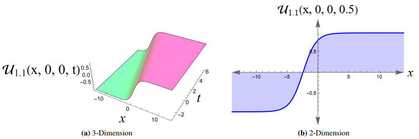
Higher-order nonlinear partial differential equations, such as the eighth-order Kac-Wakimoto model, are useful for studying wave turbulence in fluids, where energy transfers across a range of wave numbers. This phenomenon is observed in oceanographic research involving sea surface and internal waves, where intricate multi-dimensional interactions play a crucial role. In this work, we use the improved modified extended tanh function method for the first time to extract the exact solutions of the eighth-order (3+1)-dimensional Kac-Wakimoto equation, which describes the dynamics of fields and the structure of solutions in various physical and mathematical contexts. The proposed method is simple and quick to execute, and it offers more innovative solutions than other methods. As a consequence, through the donation of suitable assumptions for the parameters, some new solutions for dark and singular soliton, as well as Jacobi elliptic, exponential, hyperbolic, and singular periodic forms, are developed. Furthermore, to enhance understanding, graphical representations of certain solutions are included.
Citation: Wafaa B. Rabie, Hamdy M. Ahmed, Taher A. Nofal, E. M. Mohamed. Novel analytical superposed nonlinear wave structures for the eighth-order (3+1)-dimensional Kac-Wakimoto equation using improved modified extended tanh function method[J]. AIMS Mathematics, 2024, 9(12): 33386-33400. doi: 10.3934/math.20241593
Higher-order nonlinear partial differential equations, such as the eighth-order Kac-Wakimoto model, are useful for studying wave turbulence in fluids, where energy transfers across a range of wave numbers. This phenomenon is observed in oceanographic research involving sea surface and internal waves, where intricate multi-dimensional interactions play a crucial role. In this work, we use the improved modified extended tanh function method for the first time to extract the exact solutions of the eighth-order (3+1)-dimensional Kac-Wakimoto equation, which describes the dynamics of fields and the structure of solutions in various physical and mathematical contexts. The proposed method is simple and quick to execute, and it offers more innovative solutions than other methods. As a consequence, through the donation of suitable assumptions for the parameters, some new solutions for dark and singular soliton, as well as Jacobi elliptic, exponential, hyperbolic, and singular periodic forms, are developed. Furthermore, to enhance understanding, graphical representations of certain solutions are included.

| [1] |
A. M. Wazwaz, Two forms of (3+1)-dimensional B-type Kadomtsev-Petviashvili equation: multiple soliton solutions, Phys. Scr., 86 (2012), 035007. https://doi.org/10.1088/0031-8949/86/03/035007 doi: 10.1088/0031-8949/86/03/035007

|
| [2] |
U. Demirbilek, M. Nadeem, F. M. Çelik, H. Bulut, M. Şenol, Generalized extended (2+1)-dimensional Kadomtsev-Petviashvili equation in fluid dynamics: analytical solutions, sensitivity and stability analysis, Nonlinear Dyn., 112 (2024), 13393–13408. https://doi.org/10.1007/s11071-024-09724-3 doi: 10.1007/s11071-024-09724-3
|
| [3] |
Y. Yıldırım, Optical soliton molecules of Manakov model by trial equation technique, Optik, 185 (2019), 1146–1151. https://doi.org/10.1016/j.ijleo.2019.04.041 doi: 10.1016/j.ijleo.2019.04.041
|
| [4] |
W. B. Rabie, H. M. Ahmed, A. R. Seadawy, A. Althobaiti, The higher-order nonlinear Schrödinger's dynamical equation with fourth-order dispersion and cubic-quintic nonlinearity via dispersive analytical soliton wave solutions, Opt. Quantum Electron., 53 (2021), 1–25. https://doi.org/10.1007/s11082-021-03278-z doi: 10.1007/s11082-021-03278-z
|
| [5] |
H. U. Rehman, A. U. Awan, A. M. Hassan, S. Razzaq, Analytical soliton solutions and wave profiles of the (3+1)-dimensional modified Korteweg-de Vries-Zakharov-Kuznetsov equation, Results Phys., 52 (2023), 106769. https://doi.org/10.1016/j.rinp.2023.106769 doi: 10.1016/j.rinp.2023.106769
|
| [6] |
P. Albayrak, Optical solitons of Biswas-Milovic model having spatio-temporal dispersion and parabolic law via a couple of Kudryashov's schemes, Optik, 279 (2023), 170761. https://doi.org/10.1016/j.ijleo.2023.170761 doi: 10.1016/j.ijleo.2023.170761
|
| [7] |
M. Borg, N. M. Badra, H. M. Ahmed, W. B. Rabie, Solitons behavior of Sasa-Satsuma equation in birefringent fibers with Kerr law nonlinearity using extended F-expansion method, Ain Shams Eng. J., 15 (2024), 102290. https://doi.org/10.1016/j.asej.2023.102290 doi: 10.1016/j.asej.2023.102290
|
| [8] |
Y. Yıldırım, Optical solitons to Sasa-Satsuma model with modified simple equation approach, Optik, 184 (2019), 271–276. https://doi.org/10.1016/j.ijleo.2019.03.020 doi: 10.1016/j.ijleo.2019.03.020
|
| [9] |
A. A. Al Qarni, A. M. Bodaqah, A. S. H. F. Mohammed, A. A. Alshaery, H. O. Bakodah, A. Biswas, Cubic-quartic optical solitons for Lakshmanan-Porsezian-Daniel equation by the improved Adomian decomposition scheme, Ukr. J. Phys. Opt., 23 (2022), 228–242. https://doi.org/10.3116/16091833/23/4/228/2022 doi: 10.3116/16091833/23/4/228/2022
|
| [10] |
W. B. Rabie, H. M. Ahmed, A. Darwish, H. H. Hussein, Construction of new solitons and other wave solutions for a concatenation model using modified extended tanh-function method, Alex. Eng. J., 74 (2023), 445–451. https://doi.org/10.1016/j.aej.2023.05.046 doi: 10.1016/j.aej.2023.05.046
|
| [11] |
L. Akinyemi, H. Rezazadeh, Q. H. Shi, M. Inc, M. M. Khater, H. Ahmad, A. Jhangeer, M. A. Akbar, New optical solitons of perturbed nonlinear Schrödinger-Hirota equation with spatio-temporal dispersion, Results Phys., 29 (2021), 104656. https://doi.org/10.1016/j.rinp.2021.104656 doi: 10.1016/j.rinp.2021.104656
|
| [12] |
W. B. Rabie, H. M. Ahmed, Cubic-quartic solitons perturbation with couplers in optical metamaterials having triple-power law nonlinearity using extended F-expansion method, Optik, 262 (2022), 169255. https://doi.org/10.1016/j.ijleo.2022.169255 doi: 10.1016/j.ijleo.2022.169255
|
| [13] |
A. R. Seadawy, Approximation solutions of derivative nonlinear Schrödinger equation with computational applications by variational method, Eur. Phys. J. Plus, 130 (2015), 1–10. https://doi.org/10.1140/epjp/i2015-15182-5 doi: 10.1140/epjp/i2015-15182-5
|
| [14] |
M. S. Ghayad, N. M. Badra, H. M. Ahmed, W. B. Rabie, M. Mirzazadeh, M. S. Hashemi, Highly dispersive optical solitons in fiber Bragg gratings with cubic quadratic nonlinearity using improved modified extended tanh-function method, Opt. Quantum Electron., 56 (2024), 1184. https://doi.org/10.1007/s11082-024-07064-5 doi: 10.1007/s11082-024-07064-5
|
| [15] |
J. Yang, Y. Zhu, W. Qin, S. H. Wang, C. Q. Dai, J. T. Li, Higher-dimensional soliton structures of a variable-coefficient Gross-Pitaevskii equation with the partially nonlocal nonlinearity under a harmonic potential, Nonlinear Dyn., 108 (2022), 2551–2562. https://doi.org/10.1007/s11071-022-07337-2 doi: 10.1007/s11071-022-07337-2
|
| [16] |
H. P. Zhu, Y. J. Xu, High-dimensional vector solitons for a variable-coefficient partially nonlocal coupled Gross-Pitaevskii equation in a harmonic potential, Appl. Math. Lett., 124 (2022), 107701. https://doi.org/10.1016/j.aml.2021.107701 doi: 10.1016/j.aml.2021.107701
|
| [17] |
X. Y. Yan, J. Z. Liu, X. P. Xin, Soliton solutions and lump-type solutions to the (2+1)-dimensional Kadomtsev-Petviashvili equation with variable coefficient, Phys. Lett. A, 457 (2023), 128574. https://doi.org/10.1016/j.physleta.2022.128574 doi: 10.1016/j.physleta.2022.128574
|
| [18] | X. Y. Wu, Y. Sun, Dynamic mechanism of nonlinear waves for the (3+1)-dimensional generalized variable-coefficient shallow water wave equation, Phys. Scr., 97 (2022), 095208. https://doi.org/10.1088/1402-4896/ac878d |
| [19] |
O. D. Adeyemo, C. M. Khalique, Dynamical soliton wave structures of one-dimensional Lie subalgebras via group-invariant solutions of a higher-dimensional soliton equation with various applications in ocean physics and mechatronics engineering, Commun. Appl. Math. Comput., 4 (2022), 1531–1582. https://doi.org/10.1007/s42967-022-00195-0 doi: 10.1007/s42967-022-00195-0
|
| [20] |
A. A. Hamed, S. Shamseldeen, M. S. Abdel Latif, H. M. Nour, Analytical soliton solutions and modulation instability for a generalized (3+1)-dimensional coupled variable-coefficient nonlinear Schrödinger equations in nonlinear optics, Modern Phys. Lett. B, 35 (2021), 2050407. https://doi.org/10.1142/S0217984920504072 doi: 10.1142/S0217984920504072
|
| [21] | S. Kumar, B. Mohan, A study of multi-soliton solutions, breather, lumps, and their interactions for Kadomtsev-Petviashvili equation with variable time coeffcient using Hirota method, Phys. Scr., 96 (2021), 125255. |
| [22] | D. S. Wang, L. H. Piao, N. Zhang, Some new types of exact solutions for the Kac-Wakimoto equation associated with $\mathfrak{e}_6^{(1)}$, Phys. Scr., 95 (2020), 035202. |
| [23] |
M. Singh, Infinite-dimensional symmetry group, Kac-Moody-Virasoro algebras and integrability of Kac-Wakimoto equation, Pramana, 96 (2022), 200. https://doi.org/10.1007/s12043-022-02445-5 doi: 10.1007/s12043-022-02445-5
|
| [24] |
S. Singh, K. Sakkaravarthi, K. Manikandan, R. Sakthivel, Superposed nonlinear waves and transitions in a (3+1)-dimensional variable-coefficient eight-order nonintegrable Kac-Wakimoto equation, Chaos Solitons Fract., 185 (2024), 115057. https://doi.org/10.1016/j.chaos.2024.115057 doi: 10.1016/j.chaos.2024.115057
|
| [25] |
Z. H. Yang, B. Y. Hon, An improved modified extended tanh-function method, Z. Naturforschung A, 61 (2006), 103–115. https://doi.org/10.1515/zna-2006-3-401 doi: 10.1515/zna-2006-3-401
|
| [26] |
K. K. Ahmed, N. M. Badra, H. M. Ahmed, W. B. Rabie, Soliton solutions and other solutions for Kundu-Eckhaus equation with quintic nonlinearity and Raman effect using the improved modified extended tanh-function method, Mathematics, 10 (2022), 1–11. https://doi.org/10.3390/math10224203 doi: 10.3390/math10224203
|


Figures(4)

Wafaa B. Rabie, Hamdy M. Ahmed, Taher A. Nofal, E. M. Mohamed. Novel analytical superposed nonlinear wave structures for the eighth-order (3+1)-dimensional Kac-Wakimoto equation using improved modified extended tanh function method[J]. AIMS Mathematics, 2024, 9(12): 33386-33400. doi: 10.3934/math.20241593


 DownLoad: