Analysis of rumor spreading with different usage ranges in a multilingual environment

Liuqin Huang; Jinling Wang; Jiarong Li; Tianlong Ma; Liuqin Huang; Jinling Wang; Jiarong Li; Tianlong Ma

doi:10.3934/math.20241168

AIMS Mathematics

2024, Volume 9, Issue 9: 24018-24038. doi: 10.3934/math.20241168

Previous Article Next Article

Research article Special Issues

Analysis of rumor spreading with different usage ranges in a multilingual environment

1.
College of Mathematics and Statistics, Northwest Normal University, Lanzhou 730070, China
2.
Department of Automation, Shanghai Jiao Tong University, Shanghai 200240, China
3.
School of Sciences, Jimei University, Xiamen 361021, China

Received: 21 June 2024 Revised: 01 August 2024 Accepted: 08 August 2024 Published: 13 August 2024
MSC : 34D05, 37N20

This paper investigates rumor propagation in a multilingual environment, taking into account language usage variations. Firstly, a 2I2S2R model is proposed within a heterogeneous network framework that incorporates both immunologic and cross-transmitted mechanisms. Secondly, the paper calculates the basic reproduction number $ R_0 $ by the next-generation matrix method. Thirdly, the local asymptotic stability and the global asymptotic stability are further explored, which indicate that whether the rumor continuously spreads or becomes extinct is determined by the threshold. Finally, the numerical simulation and sensitivity analysis are given to illustrate the effectiveness of theoretical results and the influence of model parameters on rumor spreading.
- rumor spreading,
- heterogeneous network,
- multi-lingual environment,
- stability analysis
Citation: Liuqin Huang, Jinling Wang, Jiarong Li, Tianlong Ma. Analysis of rumor spreading with different usage ranges in a multilingual environment[J]. AIMS Mathematics, 2024, 9(9): 24018-24038. doi: 10.3934/math.20241168

Related Papers:

Abstract

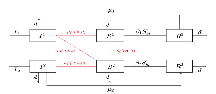
This paper investigates rumor propagation in a multilingual environment, taking into account language usage variations. Firstly, a 2I2S2R model is proposed within a heterogeneous network framework that incorporates both immunologic and cross-transmitted mechanisms. Secondly, the paper calculates the basic reproduction number $ R_0 $ by the next-generation matrix method. Thirdly, the local asymptotic stability and the global asymptotic stability are further explored, which indicate that whether the rumor continuously spreads or becomes extinct is determined by the threshold. Finally, the numerical simulation and sensitivity analysis are given to illustrate the effectiveness of theoretical results and the influence of model parameters on rumor spreading.

References

[1]	D. J. Daley, D. G. Kendall, Stochastic rumours, IMA J. Appl. Math., 1 (1965), 42–55. https://doi.org/10.1093/imamat/1.1.42 doi: 10.1093/imamat/1.1.42
[2]	L. Zhu, Y. Wang, Rumor spreading model with noise interference in complex social networks, Phys. A: Stat. Mech. Appl., 469 (2017), 750–760. https://doi.org/10.1016/j.physa.2016.11.119 doi: 10.1016/j.physa.2016.11.119
[3]	L. Zhao, J. Wang, Y. Chen, Q. Wang, J. Cheng, H. Cui, SIHR rumor spreading model in social networks, Phys. A: Stat. Mech. Appl., 391 (2012), 2444–2453. https://doi.org/10.1016/j.physa.2011.12.008 doi: 10.1016/j.physa.2011.12.008
[4]	A. Jain, J. Dhar, V. Gupta, Stochastic model of rumor propagation dynamics on homogeneous social network with expert interaction and fluctuations in contact transmissions, Phys. A: Stat. Mech. Appl., 519 (2019), 227–236. https://doi.org/10.1016/j.physa.2018.11.051 doi: 10.1016/j.physa.2018.11.051
[5]	Y. Xiao, Q. Yang, C. Sang, Y. Liu, Rumor diffusion model based on representation learning and anti-rumor, IEEE Trans. Netw. Serv. Manage., 17 (2020), 1910–1923. https://doi.org/10.1109/TNSM.2020.2994141 doi: 10.1109/TNSM.2020.2994141
[6]	D. Li, Y. Zhao, Y. Deng, Rumor spreading model with a focus on educational impact and optimal control, Nonlinear Dyn., 112 (2024), 1575–1597. https://doi.org/10.1007/s11071-023-09102-5 doi: 10.1007/s11071-023-09102-5
[7]	Z. Yu, S. Lu, D. Wang, Z. Li, Modeling and analysis of rumor propagation in social networks, Infor. Sci., 580 (2021), 857–873. https://doi.org/10.1016/j.ins.2021.09.012 doi: 10.1016/j.ins.2021.09.012
[8]	W. Pan, W. Yan, Y. Hu, R. He, L. Wu, Dynamic analysis of a SIDRW rumor propagation model considering the effect of media reports and rumor refuters, Nonlinear Dyn., 111 (2023), 3925–3936. https://doi.org/10.1007/s11071-022-07947-w doi: 10.1007/s11071-022-07947-w
[9]	Z. Zhang, X. Mei, H. Jiang, X. Luo, Y. Xia, Dynamical analysis of Hyper-SIR rumor spreading model, Appl. Math. Comput., 446 (2023), 127887. https://doi.org/10.1016/j.amc.2023.127887 doi: 10.1016/j.amc.2023.127887
[10]	Q. Liu, T. Li, M. Sun, The analysis of an SEIR rumor propagation model on heterogeneous network, Phys. A: Stat. Mech. Appl., 469 (2017), 372–380. https://doi.org/10.1016/j.physa.2016.11.067 doi: 10.1016/j.physa.2016.11.067
[11]	X. Tong, H. Jiang, J. Qiu, X. Luo, S. Chen, Dynamic analysis of the IFCD rumor propagation model under stochastic disturbance on heterogeneous networks, Chaos Soliton. Fract., 173 (2023), 113637. https://doi.org/10.1016/j.chaos.2023.113637 doi: 10.1016/j.chaos.2023.113637
[12]	J. Li, H. Jiang, X. Mei, C. Hu, G. Zhang, Dynamical analysis of rumor spreading model in multi-lingual environment and heterogeneous complex networks, Inform. Sci., 536 (2020), 391–408. https://doi.org/10.1016/j.ins.2020.05.037 doi: 10.1016/j.ins.2020.05.037
[13]	L. Zhu, X. Wang, Z. Zhang, C. Lei, Spatial dynamics and optimization method for a rumor propagation model in both homogeneous and heterogeneous environment, Nonlinear Dyn., 105 (2021), 3791–3817. https://doi.org/10.1007/s11071-021-06782-9 doi: 10.1007/s11071-021-06782-9
[14]	X. Luo, H. Jiang, S. Chen, J. Li, Stability and optimal control for delayed rumor-spreading model with nonlinear incidence over heterogeneous networks, Chinese Phys. B, 32 (2023), 058702. https://doi.org/10.1088/1674-1056/acb490 doi: 10.1088/1674-1056/acb490
[15]	D. Li, W. Qian, X. Sun, D. Han, M. Sun, Rumor spreading in a dual-relationship network with diverse propagation abilities, Appl. Math. Comput., 458 (2023), 128233. https://doi.org/10.1016/j.amc.2023.128233 doi: 10.1016/j.amc.2023.128233
[16]	X. Lv, D. Fan, Q. Li, J. Wang, L. Zhou, Simplicial SIR rumor propagation models with delay in both homogeneous and heterogeneous networks, Phys. A: Stat. Mech. Appl., 627 (2023), 129131. https://doi.org/10.1016/j.physa.2023.129131 doi: 10.1016/j.physa.2023.129131
[17]	X. Zhong, Y. Yang, F. Deng, G. Liu, Rumor propagation control with anti-rumor mechanism and intermittent control strategies, IEEE Trans. Comput. Soc. Syst., 11 (2024), 2397–2409. https://doi.org/10.1109/TCSS.2023.3277465 doi: 10.1109/TCSS.2023.3277465
[18]	N. Ding, G. Guan, S. Shen, L. Zhu, Dynamical behaviors and optimal control of delayed S2IS rumor propagation model with saturated conversion function over complex networks, Commun. Nonlinear Sci. Numer. Simul., 128 (2024), 107603. https://doi.org/10.1016/j.cnsns.2023.107603 doi: 10.1016/j.cnsns.2023.107603
[19]	X. Lv, D. Fan, J. Yang, Q. Li, L. Zhou, Delay differential equation modeling of social contagion with higher-order interactions, Appl. Math. Comput., 466 (2024), 128464. https://doi.org/10.1016/j.amc.2023.128464 doi: 10.1016/j.amc.2023.128464
[20]	S. Yu, Z. Yu, H. Jiang, J. Li, Dynamical study and event-triggered impulsive control of rumor propagation model on heterogeneous social network incorporating delay, Chaos Soliton. Fract., 145 (2021), 110806. https://doi.org/10.1016/j.chaos.2021.110806 doi: 10.1016/j.chaos.2021.110806
[21]	J. Wang, H. Jiang, T. Ma, C. Hu, Global dynamics of the multi-lingual SIR rumor spreading model with cross-transmitted mechanism, Chaos Soliton. Fract., 126 (2019), 148–157. https://doi.org/10.1016/j.chaos.2019.05.027 doi: 10.1016/j.chaos.2019.05.027
[22]	J. Liao, J. Wang, J. Li, X. Jiang, The dynamics and control of a multi-lingual rumor propagation model with non-smooth inhibition mechanism, Math. Biosci. Eng., 21 (2024), 5068–5091. https://doi.org/10.3934/mbe.2024224 doi: 10.3934/mbe.2024224
[23]	S. Yu, Z. Yu, H. Jiang, X. Mei, J. Li, The spread and control of rumors in a multilingual environment, Nonlinear Dyn., 100 (2020), 2933–2951. https://doi.org/10.1007/s11071-020-05621-7 doi: 10.1007/s11071-020-05621-7
[24]	M. Ye, J. Li, H. Jiang, Dynamic analysis and optimal control of a novel fractional-order 2I2SR rumor spreading model, Nonlinear Anal.: Model. Control, 28 (2023), 1–24. https://doi.org/10.15388/namc.2023.28.32599 doi: 10.15388/namc.2023.28.32599
[25]	Y. Ding, L. Zhu, Turing instability analysis of a rumor propagation model with time delay on non-network and complex networks, Inform. Sci., 667 (2024), 120402. https://doi.org/10.1016/j.ins.2024.120402 doi: 10.1016/j.ins.2024.120402
[26]	R. Yang, B. H. Wang, J. Ren, W. J. Bai, Z. W. Shi, W. X. Wang, et al., Epidemic spreading on heterogeneous networks with identical infectivity, Phys. Lett. A, 364 (2007), 189–193. https://doi.org/10.1016/j.physleta.2006.12.021 doi: 10.1016/j.physleta.2006.12.021
[27]	R. Pastor-Satorras, A. Vespignani, Epidemic dynamics in finite size scale-free networks, Phys. Rev. E, 65 (2002), 035108. https://doi.org/10.1103/PhysRevE.65.035108 doi: 10.1103/PhysRevE.65.035108
[28]	H. Zhang, X. Fu, Spreading of epidemics on scale-ree networks with nonlinear infectivity, Nonlinear Anal., 70 (2009), 3273–3278. https://doi.org/10.1016/j.na.2008.04.031 doi: 10.1016/j.na.2008.04.031
[29]	P. Van den Driessche, J. Watmough, Reproduction numbers and sub-threshold endemic equilibria for compartmental models of disease transmission, Math. Biosci., 180 (2002), 29–48. https://doi.org/10.1016/S0025-5564(02)00108-6 doi: 10.1016/S0025-5564(02)00108-6
[30]	J. P. LaSalle, Stability theory for ordinary differential equations, J. Differ. Equations, 4 (1968), 57–65.
[31]	F. Chen, On a nonlinear nonautonomous predator-prey model with diffusion and distributed delay, J. Comput. Appl. Math., 180 (2005), 33–49. https://doi.org/10.1016/j.cam.2004.10.001 doi: 10.1016/j.cam.2004.10.001
[32]	Z. He, Z. Cai, J. Yu, X. Wang, Y. Sun, Y. Li, Cost-efficient strategies for restraining rumor spreading in mobile social networks, IEEE Trans. Veh. Technol., 66 (2016), 2789–2800. https://doi.org/10.1109/TVT.2016.2585591 doi: 10.1109/TVT.2016.2585591
[33]	Y. Xia, H. Jiang, Z. Yu, S. Yu, X. Luo, Dynamic analysis and optimal control of a reaction-diffusion rumor propagation model in multi-lingual environments, J. Math. Anal. Appl., 521 (2023), 126967. https://doi.org/10.1016/j.jmaa.2022.126967 doi: 10.1016/j.jmaa.2022.126967
[34]	J. Wang, H. Jiang, C. Hu, Z. Yu, J. Li, Stability and Hopf bifurcation analysis of multi-lingual rumor spreading model with nonlinear inhibition mechanism, Chaos Soliton. Fract., 153 (2021), 111464. https://doi.org/10.1016/j.chaos.2021.111464 doi: 10.1016/j.chaos.2021.111464
[35]	N. Chitnis, J. M. Hyman, J. M. Cushing, Determining important parameters in the spread of malaria through the sensitivity analysis of a mathematical model, Bull. Math. Biol., 70 (2008), 1272–1296. https://doi.org/10.1007/s11538-008-9299-0 doi: 10.1007/s11538-008-9299-0

Reader Comments

Your name:*

Email:*
© 2024 the Author(s), licensee AIMS Press. This is an open access article distributed under the terms of the Creative Commons Attribution License (http://creativecommons.org/licenses/by/4.0)