A faster fixed point iterative algorithm and its application to optimization problems

Hamza Bashir; Junaid Ahmad; Walid Emam; Zhenhua Ma; Muhammad Arshad; Hamza Bashir; Junaid Ahmad; Walid Emam; Zhenhua Ma; Muhammad Arshad

doi:10.3934/math.20241153

AIMS Mathematics

2024, Volume 9, Issue 9: 23724-23751. doi: 10.3934/math.20241153

Previous Article Next Article

Research article

A faster fixed point iterative algorithm and its application to optimization problems

1.
Department of Mathematics and Statistics, International Islamic University, H-10, Islamabad 44000, Pakistan
2.
Department of Statistics and Operations Research, Faculty of Science, King Saud University, P.O. Box 2455, Riyadh 11451, Saudi Arabia
3.
Department of Mathematics and Physics, Hebei University of Architecture, Zhangjiakou 075024, China

Received: 10 May 2024 Revised: 17 July 2024 Accepted: 25 July 2024 Published: 08 August 2024
MSC : 47H05, 47H09, 47H10

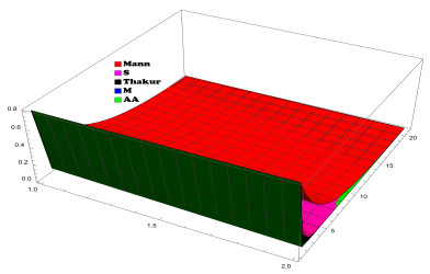
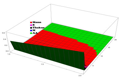
In this paper, we studied the AA-iterative algorithm for finding fixed points of the class of nonlinear generalized $ (\alpha, \beta) $-nonexpansive mappings. First, we proved weak convergence and then proved several strong convergence results of the scheme in a ground setting of uniformly convex Banach spaces. We gave a few numerical examples of generalized $ (\alpha, \beta) $-nonexpansive mappings to illustrate the major outcomes. One example was constructed over a subset of a real line while the other one was on the two dimensional space with a taxicab norm. We considered both these examples in our numerical computations to show that our iterative algorithm was more effective in the rate of convergence corresponding to other fixed point algorithms of the literature. Some 2D and 3D graphs were obtained that supported graphically our results and claims. As applications of our major results, we solved a class of fractional differential equations, 2D Voltera differential equation, and a convex minimization problem. Our findings improved and extended the corresponding results of the current literature.
- iteration,
- fixed point,
- differential equation,
- optimization problem,
- Banach space
Citation: Hamza Bashir, Junaid Ahmad, Walid Emam, Zhenhua Ma, Muhammad Arshad. A faster fixed point iterative algorithm and its application to optimization problems[J]. AIMS Mathematics, 2024, 9(9): 23724-23751. doi: 10.3934/math.20241153

Related Papers:

Abstract

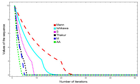
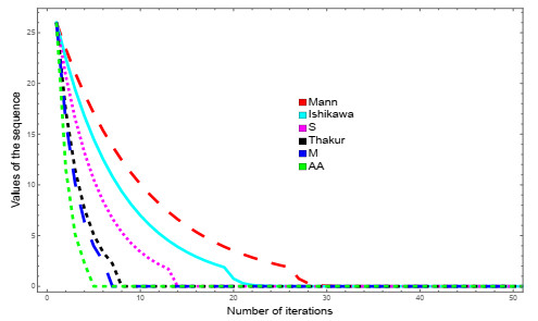
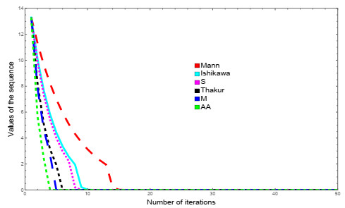
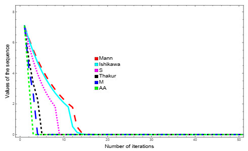
In this paper, we studied the AA-iterative algorithm for finding fixed points of the class of nonlinear generalized $ (\alpha, \beta) $-nonexpansive mappings. First, we proved weak convergence and then proved several strong convergence results of the scheme in a ground setting of uniformly convex Banach spaces. We gave a few numerical examples of generalized $ (\alpha, \beta) $-nonexpansive mappings to illustrate the major outcomes. One example was constructed over a subset of a real line while the other one was on the two dimensional space with a taxicab norm. We considered both these examples in our numerical computations to show that our iterative algorithm was more effective in the rate of convergence corresponding to other fixed point algorithms of the literature. Some 2D and 3D graphs were obtained that supported graphically our results and claims. As applications of our major results, we solved a class of fractional differential equations, 2D Voltera differential equation, and a convex minimization problem. Our findings improved and extended the corresponding results of the current literature.

References

[1]	L. M. Guo, Y. Wang, H. M. Liu, C. Li, J. B. Zhao, H. L. Chu, On iterative positive solutions for a class of singular infinite-point p-Laplacian fractional differential equations with singular source terms, J. Appl. Anal. Comput., 13 (2023), 2827–2842. https://doi.org/10.11948/20230008 doi: 10.11948/20230008
[2]	S. Banach, Sur les operations dans les ensembles abstraits et leur application aux equations integrales, Fund. Math., 3 (1922), 133–181. https://doi.org/10.4064/fm-3-1-133-181 doi: 10.4064/fm-3-1-133-181
[3]	Y. Yu, T. C. Yin, Strong convergence theorems for a nonmonotone equilibrium problem and a quasi-variational inclusion problem, J. Nonlinear Convex Anal., 25 (2024), 503–512.
[4]	W. A. Kirk, A fixed point theorem for mappings which do not increase distance, Amer. Math. Mon., 72 (1965), 1004–1006. https://doi.org/10.2307/2313345 doi: 10.2307/2313345
[5]	F. E. Browder, Nonexpansive nonlinear operators in a Banach space, Proc. Natl. Acad. Sci., 54 (1965), 1041–1044. https://doi.org/10.1073/pnas.54.4.1041 doi: 10.1073/pnas.54.4.1041
[6]	D. Gohde, Zum Prinzip der Kontraktiven Abbildung, Math. Nachr., 30 (1965), 251–258. https://doi.org/10.1002/mana.19650300312 doi: 10.1002/mana.19650300312
[7]	T. Suzuki, Fixed point theorems and convergence theorems for some generalized non-expansive mapping, J. Math. Anal. Appl., 340 (2008), 1088–1095. https://doi.org/10.1016/j.jmaa.2007.09.023 doi: 10.1016/j.jmaa.2007.09.023
[8]	B. S. Thakur, D. Thakur, M. Postolache, A new iterative scheme for numerical reckoning fixed points of Suzuki's generalized nonexpansive mappings, Appl. Math. Comput., 275 (2016), 147–155. https://doi.org/10.1016/j.amc.2015.11.065 doi: 10.1016/j.amc.2015.11.065
[9]	K. Aoyama, F. Kohsaka, Fixed point theorem for $\alpha$-nonexpansive mappings in Banach spaces, Nonlineaar Anal. Theor., 74 (2011), 4387–4391. https://doi.org/10.1016/j.na.2011.03.057 doi: 10.1016/j.na.2011.03.057
[10]	H. Piri, B. Daraby, S. Rahrovi, M. Ghasemi, Approximating fixed points of generalized $\alpha$-nonexpansive mappings in Banach spaces by new faster iteration process, Numer. Algor., 81 (2019), 1129–1148. https://doi.org/10.1007/s11075-018-0588-x doi: 10.1007/s11075-018-0588-x
[11]	R. Pant, R. Shukla, Approximating fixed points of generalized $\alpha$-nonexpansive mappings in Banach spaces, Numer. Funct. Anal. Opt., 38 (2017), 248–266. https://doi.org/10.1080/01630563.2016.1276075 doi: 10.1080/01630563.2016.1276075
[12]	R. Shukla, R. Pant, M. De la Sen, Generalized $\alpha$-nonexpansive mappings in Banach spaces, Fixed Point Theory and Appl., 2017, (2016), 4. https://doi.org/10.1186/s13663-017-0597-9 doi: 10.1186/s13663-017-0597-9
[13]	R. Pant, R. Pandey, Existence and convergence results for a class of nonexpansive type mappings in hyperbolic spaces, Appl. Gen. Topol., 20 (2019), 281–295. https://doi.org/10.4995/agt.2019.11057 doi: 10.4995/agt.2019.11057
[14]	K. Ullah, J. Ahmad, M. De La Sen, On generalized nonexpansive maps in Banach spaces, Computation, 8 (2020), 61. https://doi.org/10.3390/computation8030061 doi: 10.3390/computation8030061
[15]	F. Ahmad, K. Ullah, J. Ahmad, H. Bilal, On an efficient iterative scheme for a class of generalized nonexpansive operators in Banach spaces, Asian-Eur. J. Math., 16 (2023), 2350172. https://doi.org/10.1142/S1793557123501723 doi: 10.1142/S1793557123501723
[16]	M. Yang, J. Sun, Z. Fu, Z. Wang, The singular convergence of a Chemotaxis-Fluid system modeling coral fertilization, Acta. Math. Sci., 43, (2023), 492–504. https://doi.org/10.1007/s10473-023-0202-8 doi: 10.1007/s10473-023-0202-8
[17]	S. Shi, Z. Zhai, L. Zhang, Characterizations of the viscosity solution of a nonlocal and nonlinear equation induced by the fractional p-Laplace and the fractional p-convexity, Adv. Calc. Var., 17 (2024), 195–207. https://doi.org/10.1515/acv-2021-0110 doi: 10.1515/acv-2021-0110
[18]	W. R. Mann, Mean value methods in iteration, Proc. Amer. Math. Soc., 4 (1953), 506–510. https://doi.org/10.1090/S0002-9939-1953-0054846-3 doi: 10.1090/S0002-9939-1953-0054846-3
[19]	S. Ishikawa, Fixed points by a new iteration method, Proc. Amer. Math. Soc., 44 (1974), 147–150. https://doi.org/10.1090/S0002-9939-1974-0336469-5 doi: 10.1090/S0002-9939-1974-0336469-5
[20]	M. A. Noor, New approximation schemes for general variational inequalities, J. Math. Anal. Appl., 251 (2000), 217–229. https://doi.org/10.1006/jmaa.2000.7042 doi: 10.1006/jmaa.2000.7042
[21]	R. P. Agarwal, D. O'Regon, D. R. Sahu, Iterative construction of fixed points of nearly asymptotically nonexpansive mappings, J. Nonlinear Convex Anal., 8 (2007), 61–79.
[22]	M. Abbas, T. Nazir, A new faster iteration process applied to constrained minimization and feasibility problems, Mat. Vestn., 66 (2014), 223–234.
[23]	N. Hussain, K. Ullah, M. Arshad, Fixed point approximation of Suzuki generalized nonexpansive mappings via new faster iteration process, J. Nonlinear Convex Anal., 19 (2018), 1383–1393.
[24]	K. Ullah, J. Ahmad, F. M. Khan, Numerical reckoning fixed points via new faster iteration process, Appl. Gen. Topol., 23 (2022), 213–223. https://doi.org/10.4995/agt.2022.11902 doi: 10.4995/agt.2022.11902
[25]	M. Abbas, M. W. Asghar, M. De la Sen, Approximation of the solution of delay fractional differential equation using AA-Iterative Scheme, Mathematics, 10 (2022), 273. https://doi.org/10.3390/math10020273 doi: 10.3390/math10020273
[26]	J. Ali, F. Ali, P. Kumar, Approximation of fixed points for Suzuki's generalized nonexpansive mappings, Mathematics, 7 (2019), 522. https://doi.org/10.3390/math7060522 doi: 10.3390/math7060522
[27]	Z. Ma, H. Bashir, A. A. Alshejari, J. Ahmad, M. Arshad, An algorithm for nonlinear problems based on fixed point methodologies with applications, Int. J. Anal. Appl., 22 (2024), 77. https://doi.org/10.28924/2291-8639-22-2024-77 doi: 10.28924/2291-8639-22-2024-77
[28]	J. A. Clarkson, Uniformly convex spaces, Trans. Amer. Math. Soc., 40 (1936), 396–414. https://doi.org/10.1090/S0002-9947-1936-1501880-4 doi: 10.1090/S0002-9947-1936-1501880-4
[29]	Z. Opial, Weak convergence of the sequence of successive approximations for nonexpansive mappings, Bull. Amer. Math. Soc., 73 (1967), 591–597. https://doi.org/10.1090/S0002-9904-1967-11761-0 doi: 10.1090/S0002-9904-1967-11761-0
[30]	W. Takahashi, Nonlinear functional analysis, Yokohoma: Yokohoma Publishers, 2000.
[31]	H. F. Senter, W. G. Dotson, Approximating fixed points of nonexpansive mappings, Proc. Amer. Math. Soc., 44 (1974), 375–380. https://doi.org/10.1090/S0002-9939-1974-0346608-8 doi: 10.1090/S0002-9939-1974-0346608-8
[32]	J. Schu, Weak and strong convergence to fixed points of asymptotically nonexpansive mappings, Bull. Aust. Math. Soc., 43 (1991), 153–159. https://doi.org/10.1017/S0004972700028884 doi: 10.1017/S0004972700028884
[33]	E. Karapnar, T. Abdeljawad, F. Jarad, Applying new fixed point theorems on fractional and ordinary differential equations, Adv. Differ. Equ., 2019 (2019), 421. https://doi.org/10.1186/s13662-019-2354-3 doi: 10.1186/s13662-019-2354-3

Reader Comments

Your name:*

Email:*
© 2024 the Author(s), licensee AIMS Press. This is an open access article distributed under the terms of the Creative Commons Attribution License (http://creativecommons.org/licenses/by/4.0)