A review of different deep learning techniques for sperm fertility prediction

Muhammad Suleman; Muhammad Ilyas; M. Ikram Ullah Lali; Hafiz Tayyab Rauf; Seifedine Kadry; Muhammad Suleman; Muhammad Ilyas; M. Ikram Ullah Lali; Hafiz Tayyab Rauf; Seifedine Kadry

doi:10.3934/math.2023838

AIMS Mathematics

2023, Volume 8, Issue 7: 16360-16416. doi: 10.3934/math.2023838

Previous Article Next Article

Review Special Issues

A review of different deep learning techniques for sperm fertility prediction

1.
Department of CS IT, University of Sargodha, Pakistan
2.
Department of Information Sciences, University of Education Lahore, Pakistan
3.
Independent Researcher, UK
4.
Department of Applied Data Science, Noroff University College, Kristiansand, Norway
5.
Artificial Intelligence Research Center (AIRC), College of Engineering and Information Technology, Ajman University, Ajman, United Arab Emirates
6.
Department of Electrical and Computer Engineering, Lebanese American University, Byblos, Lebanon

Received: 02 January 2023 Revised: 15 April 2023 Accepted: 17 April 2023 Published: 08 May 2023
MSC : 68T07

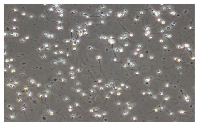
Sperm morphology analysis (SMA) is a significant factor in diagnosing male infertility. Therefore, healthy sperm detection is of great significance in this process. However, the traditional manual microscopic sperm detection methods have the disadvantages of a long detection cycle, low detection accuracy in large orders, and very complex fertility prediction. Therefore, it is meaningful to apply computer image analysis technology to the field of fertility prediction. Computer image analysis can give high precision and high efficiency in detecting sperm cells. In this article, first, we analyze the existing sperm detection techniques in chronological order, from traditional image processing and machine learning to deep learning methods in segmentation and classification. Then, we analyze and summarize these existing methods and introduce some potential methods, including visual transformers. Finally, the future development direction and challenges of sperm cell detection are discussed. We have summarized 44 related technical papers from 2012 to the present. This review will help researchers have a more comprehensive understanding of the development process, research status, and future trends in the field of fertility prediction and provide a reference for researchers in other fields.

Keywords:

sperm morphology,
automatic image analysis,
sperm defects,
infertility, Convolutional Neural Network (CNN), deep learning

Citation: Muhammad Suleman, Muhammad Ilyas, M. Ikram Ullah Lali, Hafiz Tayyab Rauf, Seifedine Kadry. A review of different deep learning techniques for sperm fertility prediction[J]. AIMS Mathematics, 2023, 8(7): 16360-16416. doi: 10.3934/math.2023838

Related Papers:

[1]	Taekyun Kim, Dae San Kim, Jin-Woo Park . Degenerate $r$ -truncated Stirling numbers. AIMS Mathematics, 2023, 8(11): 25957-25965. doi: 10.3934/math.20231322
[2]	Taekyun Kim, Dae San Kim, Hyunseok Lee, Lee-Chae Jang . A note on degenerate derangement polynomials and numbers. AIMS Mathematics, 2021, 6(6): 6469-6481. doi: 10.3934/math.2021380
[3]	Dojin Kim, Patcharee Wongsason, Jongkyum Kwon . Type 2 degenerate modified poly-Bernoulli polynomials arising from the degenerate poly-exponential functions. AIMS Mathematics, 2022, 7(6): 9716-9730. doi: 10.3934/math.2022541
[4]	Dae San Kim, Hye Kyung Kim, Taekyun Kim . New approach to $\lambda$ -Stirling numbers. AIMS Mathematics, 2023, 8(12): 28322-28333. doi: 10.3934/math.20231449
[5]	Sang Jo Yun, Jin-Woo Park . On a generation of degenerate Daehee polynomials. AIMS Mathematics, 2025, 10(5): 12286-12298. doi: 10.3934/math.2025556
[6]	Aimin Xu . Some identities connecting Stirling numbers, central factorial numbers and higher-order Bernoulli polynomials. AIMS Mathematics, 2025, 10(2): 3197-3206. doi: 10.3934/math.2025148
[7]	Feng Qi, Da-Wei Niu, Bai-Ni Guo . Simplifying coefficients in differential equations associated with higher order Bernoulli numbers of the second kind. AIMS Mathematics, 2019, 4(2): 170-175. doi: 10.3934/math.2019.2.170
[8]	Taekyun Kim, Dae San Kim, Dmitry V. Dolgy, Hye Kyung Kim, Hyunseok Lee . A new approach to Bell and poly-Bell numbers and polynomials. AIMS Mathematics, 2022, 7(3): 4004-4016. doi: 10.3934/math.2022221
[9]	Hye Kyung Kim . Note on $r$ -central Lah numbers and $r$ -central Lah-Bell numbers. AIMS Mathematics, 2022, 7(2): 2929-2939. doi: 10.3934/math.2022161
[10]	Letelier Castilla, William Ramírez, Clemente Cesarano, Shahid Ahmad Wani, Maria-Fernanda Heredia-Moyano . A new class of generalized Apostol–type Frobenius–Euler polynomials. AIMS Mathematics, 2025, 10(2): 3623-3641. doi: 10.3934/math.2025167

Abstract

1. Introduction

Many people with physical mobility impairments, such as spinal and multiple sclerosis, need to use intelligent wheelchairs for various activities in their surroundings ^[1,2,3]. Conventional wheelchairs may meet the specific needs of some patients, but most patients, however, need to use innovative chairs with advanced technologies that use smart devices and consider various safety measures ^[4]. Recent decades have seen significant advances in developing control technologies for autonomous and semi-autonomous wheelchairs. These developments have been characterized by improving comfort, safety and driving in an ideal way while avoiding obstacles in different conditions, depending on the supervisory control based on the sensory systems and the user's intention. These developments also included using smartphones, developing navigation algorithms, hands-free driving and sharing users' locations to improve system performance conditions ^[3,4].

In general, driving-level control technologies of mobile wheelchairs have been divided into two categories. The supervisory category operates the mobile wheelchairs to perform intelligent tasks, such as avoiding obstacles and following a given path, and are essential to optimum performance ^[5]. The low-level category needs to be developed to raise the level of fine motion control. This is because this level of control deals with many variables that need to design numerical algorithms for the designed systems. Therefore, this kind of research needs to develop efficient algorithms that deal with system uncertainties and external perturbations ^[6]. Nevertheless, there has been a lack of emphasis among researchers on the specific category of low-level control.

Various low-level control techniques have been proposed for driving smart wheelchairs, including proportional-derivative (PD) controller, fuzzy logic control (FLC), sliding mode control (SMC) ^[7], adaptive neural network of nonsingular terminal sliding mode control ^[8], quasi linear parameter varying control ^[9], H-infinity ^[10], Lagrangien method with FLC ^[11], and backstepping control with a proportional-integral-derivative (PID) controller ^[12]. However, the majority of these haven't considered the motorized wheelchair to be a multivariate system. The challenge of setting the control design into action for a multivariate system can be difficult because of the interactions between the various inputs and outputs of the system. The problems inherently present in a multivariate system can frequently be resolved using separation techniques, which are very effective solutions. These methods attempt to alleviate the complexity of the problem of multivariate control by breaking it down into several separate numerical control issues. Nevertheless, there has yet to be a lot of research done looking at how durable systems are when subjected to the influence of uncertainty and external perturbations.

Recently, a model reference control method for a semi-autonomous powered wheelchair has been proposed and evaluated in different condition states. This method adopted quasi-linear closed-loop behavior as a control loop to achieve robustness. To mitigate modeling uncertainties, the technique also compensated for non-linear dynamics associated with a veer rate ^[13]. A digital control and encoding method was also introduced to obtain real-time robustness tracking in smart wheelchairs. The method utilized PID with an open-loop controller to vary the speed in different proposed surfaces. Experimental results demonstrated that this method was effective in proposed surfaces using different speeds ^[14]. Another method conducted by Seki and Tanohata ^[15] implemented an FLC algorithm based on a torque scheme to drive a wheelchair on a disturbance road. In this approach, the algorithm was developed by incorporating human input torque and driving velocity. The effectiveness of this method was evaluated utilizing a real-time experimental test, and the results depicted that this control method was robust on driving on disturbance roads. Despite the evaluations made on these methods, they face several challenges in appropriately addressing the changing parameters of the system and effectively mitigating the impact of noise.

The neural network approach is one of the control tools that have been developed recently to control linear and nonlinear systems. This is done by providing it with many effective characteristics, such as the ability to generalize through experience for many planned and nonlinear inputs. This approach provided the ability to devise different ways to overcome noise and multivariate interactions. Neural networks have demonstrated efficacy in addressing complicated control operations by designing structures for those networks used in solving arithmetic sequences ^[16]. For instance, Aly et al. ^[17] developed a tracking control algorithm for the upper-limb exoskeleton using an adaptive neural backstepping in the presence of external disturbance and model uncertainty. The Lyapunov stability was obtained to achieve the system parameter convergence while evaluating the designed algorithm. The findings from the simulation study indicated that the proposed methodology effectively monitored and mitigated disturbances and uncertainties in the model. The control method for the upper-limb exoskeleton, as presented by the authors in reference [8], involved the utilization of an adaptive neural network based on fixed-time tracking. This approach incorporated an integral nonsingular terminal sliding mode. The method was evaluated using MATLAB simulink tools (The MathWorks Inc., Natick, USA), and the results show that the technique was effective in the presence of external disturbance and model uncertainty. However, the upper proposed methods were only in silico evaluated and updated, so this kind of control law is still complicated.

This paper addresses a number of challenging issues associated with the trajectory tracking control of mobile wheelchairs. This is related to stability and tracking performance, where precise trajectory monitoring is essential for advancing autonomy guidance. Therefore, this work aims to design an efficient method to track the reference trajectory in the presence of disturbances or system parameter variation. The proposed technique employed the neural pole placement sliding mode control (PP-SMC) method to achieve the system robustness. The stability analysis was studied, and the numerical evaluation approach was conducted using MATLAB simulink tools to demonstrate the system's performance. To our knowledge, this is the first study in which the placement method combined with a neural sliding mode that adopted the Gao reaching law has been employed to control the low-level dynamic model of mobile wheelchairs.

2. Materials and methods

2.1. Dynamical model

As shown in , the nonlinear dynamic system model of the mobile wheelchair can be described in the form of cartesian coordinates ( ${\chi _w}＆ {y_w}$ ) and the mobile orientation ( $\Phi$ ) ^[18]. In this model, the center of mass is denoted by ( $H$ ), and the distance between $H$ and the central point of the virtual axis ( $G$ ) is denoted by ( $l$ ). As a result, the updated kinematic model can be illustrated as:

$\left[ {\begin{array}{*{20}{c}} {\dot \chi \left( t \right)} \\ {\dot y\left( t \right)} \end{array}} \right] = \left[ {\begin{array}{*{20}{c}} {\begin{array}{*{20}{c}} {\cos \Phi \left( t \right)}&{ - l\sin \Phi \left( t \right)} \end{array}} \\ {\begin{array}{*{20}{c}} {\sin \Phi \left( t \right)}&{l\cos \Phi \left( t \right)} \end{array}} \end{array}} \right]\left[ {\begin{array}{*{20}{c}} {{u_1}\left( t \right)} \\ {{u_2}\left( t \right)} \end{array}} \right] + \left[ {\begin{array}{*{20}{c}} {{\gamma _x}\left( t \right)} \\ {{\gamma _y}\left( t \right)} \end{array}} \right],$

(1)

Figure 1. Kinematic controlled model.

DownLoad: Full-Size Img PowerPoint

where $\chi \in {R^n}$ is the state vector of the dynamic system,

$u = \left[ {\begin{array}{*{20}{c}} {{u_1}\left( t \right)} \\ {{u_2}\left( t \right)} \end{array}} \right] \in {R^m}$

is the input vector, $\gamma \left(t \right)$ is the system disturbance,

$y = \left[ {\begin{array}{*{20}{c}} {\upsilon \left( t \right)} \\ {\omega \left( t \right)} \end{array}} \right]$

is the model output of linear velocity (v(t)) and angular velocity (ω(t)).

The dynamic output model is calculated based on the following equations:

$\left\{ {\begin{array}{*{20}{c}} {\upsilon \left( t \right) = {{R\left( {{\omega _r} + {\omega _l}} \right)} \mathord{\left/ {\vphantom {{R\left( {{\omega _r} + {\omega _l}} \right)} 2}} \right. } 2}, } \\ {\omega \left( t \right) = R{{\left( {{\omega _r} - {\omega _l}} \right)} \mathord{\left/ {\vphantom {{\left( {{\omega _r} - {\omega _l}} \right)} {D, }}} \right. } {D, }}} \end{array}} \right.$

(2)

here ${\omega _r}＆ {\omega _l}$ are right and left of angular velocities, D is the distance between the wheels, and R is the right and left wheel radius.

By using the Euler-Lagrangian approach ^[19], the dynamic model in (1) can be expressed as follows:

$\begin{gathered} \dot \chi (t) = \left( {a + \delta a} \right)\chi (t) + bu(t) + \gamma \left( t \right), \hfill \\ \dot y(t) = c\chi (t), \hfill \\ \end{gathered}$

(3)

where, $\delta a$ is the system parameter variation, $\gamma \left(t \right)$ is the system disturbance and a, b and c are matrices with compatible dimensioning.

2.2. Controller design

Consider the dynamic model in (3) is without uncertainty and disturbance is given as:

$\begin{gathered} \dot \chi (t) = a\chi (t) + bu(t), \hfill \\ \dot y(t) = c\chi (t), \hfill \\ \end{gathered}$

(4)

and we assume that the correspondence reference model is given by:

$\dot q(t) = {a_k}q(t) + {b_k}r(t),$

(5)

where $q \in {R^n}$ is the vector that representing the states of the reference model, $r \in {R^i}$ is an input vector for reference model and ( ${a_k}＆ {b_k}$ ) are compatibly dimensioned matrices.

2.2.1. Pole placement method

For the sake of implementing this strategy, we are assuming that the pairs (a & b) and ( ${a_k}＆ {b_k}$ ) are able to be controlled, thus demonstrating stability of the reference model. This implies that the eigenvalues of ${a_k}$ are located within the open unit disc. In order to develop the algorithm, we take into account the tractability of the model referenced in (5) by the model presented in (4). Therefore, this requires to determine the ( ${a_k}＆ {b_k}$ ) based on the following non-proofing theorem ^[20]:

Theorem 1. For any system $a\chi = c$ , where is $a \in {R^{n*m}}$ matrix and $c \in {\mathbb{R}^m}$ is a vector, there exists a solution $rank\left[ a \right] = rank\left[ {{a_c}} \right]$ if and only if ${a_c} \in m\left({n + 1} \right)$ is an augmented matrix.

Based on that we can write: $rank\left[ {\begin{array}{*{20}{c}} b & {{a_k} - a} \end{array}} \right] = rank\left[ b \right]$ ; $rank\left[ {\begin{array}{*{20}{c}} b & {{b_k}} \end{array}} \right] = rank\left[ b \right]$ , then the previous theorem has the significant conclusion that $K$ and $G$ have matrices with compatible dimensions in such a way as:

$\begin{gathered} {a_k} = a - bk, \hfill \\ {b_k} = bg, \hfill \\ \end{gathered}$

(6)

where $k = \left[ {{k_1}, {k_2}, \cdots, {k_{\text{n}}}} \right]$ , w represents the state feedback matrix generated with the pole placement method or Ackerman's formula to achieve asymptotically stable behavior in closed-loop dynamic systems.

The term $g$ represents the feedforward steady-state gain, which may be determined by finding the inverse of the triple components ( $c, \left({a + bk} \right), b$ ) as the following:

Consider that the proposed state feedback law is formulated as follows:

$u\left( t \right) = k\chi \left( t \right) + gr\left( t \right) ,$

(7)

the obtained state equation for the closed-loop system is as follows:

$\begin{gathered} \dot \chi (t) = \left( {a + bk} \right)\chi (t) + bgr(t), \hfill \\ \dot y(t) = c\chi (t). \hfill \\ \end{gathered}$

(8)

To obtain g, we assume that the reference input $r\left(t \right) = \Psi$ and the steady state output can be written as:

${y_{ss}} \equiv \mathop {\lim }\limits_{t \to \infty } y\left( t \right) = \Psi .$

(9)

For the constant $\Psi$ at $t \geqslant 0$ , the closed-loop state equation that involves an equilibrium state can satisfy the following condition:

$\dot \chi (t) = \left( {a + bk} \right){\chi _{ss}}\left( t \right) + bg\Psi = 0,$

(10)

${\chi _{ss}}(t) = c{\left( {a + bk} \right)^{ - 1}}bg\Psi .$

(11)

The steady-state output can be obtained using the following:

${y_{ss}} = c{\chi _{ss}}(t) = c{\left( {a + bk} \right)^{ - 1}}bg\Psi .$

(12)

From (9) we can write:

$\Psi = c{\left( {a + bk} \right)^{ - 1}}bg\Psi .$

(13)

As a result, the feedforward gain can be obtained as:

$g = {\left( {c{{\left( {a + bk} \right)}^{ - 1}}b} \right)^{ - 1}}.$

(14)

In this study, we define the trajectory error as:

$\begin{gathered} {e_\chi }\left( t \right) = \chi \left( t \right) - q\left( t \right), \hfill \\ {{\dot e}_\chi }\left( t \right) = \dot \chi \left( t \right) - \dot q\left( t \right). \hfill \\ \end{gathered}$

(15)

By substituting (4) and (5) in (15), we can write:

${\dot e_\chi }\left( t \right) = a\chi (t) + bu(t) - \left( {{a_k}q(t) + {b_k}r(t)} \right).$

(16)

By adding and subtracting the term ${a_k}\chi \left(t \right)$ we can get:

${\dot e_\chi }\left( t \right) = a\chi (t) + {a_k}\chi \left( t \right) - {a_k}\chi \left( t \right) + bu(t) - {a_k}q(t) - {b_k}r(t),$

(17)

${\dot e_\chi }\left( t \right) = {a_k}{e_\chi }\left( t \right) + \left( {a - {a_k}} \right)\chi \left( t \right) + bu(t) - {b_k}r(t).$

(18)

2.2.2. SMC method

In this study we employed the SMC method and chose the following switch function ^[21,22]:

$\begin{gathered} s\left( t \right) = \xi {e_\chi }\left( t \right), \hfill \\ \dot s\left( t \right) = \xi {{\dot e}_\chi }\left( t \right). \hfill \\ \end{gathered}$

(19)

By substituting (18) in (19) we can get:

$\dot s\left( t \right) = \xi \left( {{a_k}{e_\chi }\left( t \right) + \left( {a - {a_k}} \right)\chi \left( t \right) + bu(t) - {b_k}r(t)} \right) .$

(20)

To achieve a robust stability, we proposed to adopt a Gao reaching law ^[21] as:

$\dot s\left( t \right) = - \left( {\tau s\left( t \right) + \beta sign\left( {s\left( t \right)} \right)} \right),$

(21)

where, $\tau > 0$ , $\beta > 0$ and $sign\left({s\left(t \right)} \right)$ is the signum function given by:

$sign\left( {s\left( t \right)} \right) = \left\{ {\begin{array}{*{20}{c}} {\begin{array}{*{20}{c}} { + 1, }&{s\left( t \right) \geqslant 0, } \end{array}} \\ {\begin{array}{*{20}{c}} { - 1, }&{s\left( t \right) < 0.} \end{array}} \end{array}} \right.$

By equivalating (20) to (21) we can get:

$- \left( {\tau s\left( t \right) + \beta sign\left( {s\left( t \right)} \right)} \right) = \xi \left( {{a_k}{e_\chi }\left( t \right) + \left( {a - {a_k}} \right)\chi \left( t \right) + bu(t) - {b_k}r(t)} \right) .$

(22)

Solving (22) in terms of $u(t)$ we can write:

$u\left( t \right) = - {\left( {\xi b} \right)^{ - 1}}\left( \begin{gathered} \xi {a_k}{e_\chi }\left( t \right) + \xi \left( {a - {a_k}} \right)\chi \left( t \right) - \xi {b_k}r(t) \hfill \\ - \tau \xi {e_\chi }\left( t \right) - \beta sign\left( {\xi {e_\chi }\left( t \right)} \right) \hfill \\ \end{gathered} \right) .$

(23)

The model presented in (4) can be rewritten as follows when there is uncertainty in either the disturbances or the system parameters:

$\begin{gathered} \dot \chi (t) = \left( {a + \delta a} \right)\chi (t) + bu(t) + \gamma \left( t \right), \hfill \\ \dot y(t) = c\chi (t). \hfill \\ \end{gathered}$

(24)

The control algorithm in (24) can be written as:

(25)

The control algorithm ( ${u_t}(t)$ ) in (25) can be constructed as equivalent $\left({{u_{eqv}}(t)} \right)$ and corrective $\left({{u_{corr}}(t)} \right)$ parts as:

$u(t) = {u_{eqv}}(t) + {u_{corr}}(t) ,$

(26)

where,

${u_{eqv}}\left( t \right) = - {\left( {\xi b} \right)^{ - 1}}\left( \begin{gathered} \xi {a_k}{e_\chi }\left( t \right) + \xi \left( {a - {a_k}} \right)\chi \left( t \right) - \xi {b_k}r(t) \hfill \\ - \left( {\xi \delta a\chi \left( t \right) + \xi \gamma \left( t \right)} \right) \hfill \\ \end{gathered} \right),$

(27)

${u_{corr}}\left( t \right) = {\left( {\xi b} \right)^{ - 1}}\left( {\tau \xi {e_\chi }\left( t \right) + \beta sign\left( {\xi {e_\chi }\left( t \right)} \right)} \right) .$

(28)

2.2.3. Neural networks control method

Neural networks method has proposed to adjust the values varying of the system parameters and disturbances by estimating both equivalent and corrective laws ^[23]. In this method, the equivalent neural network keeps the system states on the $s\left(t \right) = 0$ , while the corrective neural network is trained to retune all states back to the proposed sliding surface. To eliminate any chattering, we proposed to replace the $\left({sign\left({s\left(t \right)} \right)} \right)$ function with

$\mu = {{\left( {1 - {e^{ - s\left( t \right)}}} \right)} \mathord{\left/ {\vphantom {{\left( {1 - {e^{ - s\left( t \right)}}} \right)} {\left( {1 + {e^{ - s\left( t \right)}}} \right)}}} \right. } {\left( {1 + {e^{ - s\left( t \right)}}} \right)}} .$

The estimated the equivalent control law is given by:

${\overset{\lower0.5em\hbox{$\smash{\scriptscriptstyle\frown}$}}{u} _{eqv}}(t) = {k_u}\mu \left( {s\left( t \right)} \right)\left( {\sum\limits_{i = 1}^m {{{\rm H}_i}.\mu \left( {s\left( t \right)} \right)\left( {\sum\limits_{j = 1}^n {{{\bar {\rm H}}_{j, i}}.{{\rm O}_i}} } \right)} } \right) .$

(29)

The estimated corrective control law as is given by:

${\overset{\lower0.5em\hbox{$\smash{\scriptscriptstyle\frown}$}}{u} _{corr}}(t) = {k_c}.\mu \left( {s\left( t \right)} \right)\left( {\sum\limits_{j = 1}^n {{\varphi _j}{e_j}\left( t \right)} } \right) .$

(30)

To obtain a robust estimation, the following cost functions were proposed:

$J = 0.5{u^2}_{eqv}(t) + {u_{eqv}}(t)*{\overset{\lower0.5em\hbox{$\smash{\scriptscriptstyle\frown}$}}{u} _{eqv}}(t) + 0.5{\overset{\lower0.5em\hbox{$\smash{\scriptscriptstyle\frown}$}}{u} ^2}_{eqv}(t) ,$

(31)

${\rm Z} = 0.5{s^2}(t) .$

(32)

Based on (31), the weight updating law to reduce $J$ can be written as:

$\Delta {{\rm H}_i} = - \beta {{\partial J} \mathord{\left/ {\vphantom {{\partial J} {\partial {{\rm H}_i} = 0.5\left( {\beta {k_u}s\left( t \right) - \beta {k_u}s\left( t \right)\mu \left( {s\left( t \right)} \right){u^2}y\left( t \right)} \right)}}} \right. } {\partial {{\rm H}_i} = 0.5\left( {\beta {k_u}s\left( t \right) - \beta {k_u}s\left( t \right)\mu \left( {s\left( t \right)} \right){u^2}y\left( t \right)} \right)}} ,$

(33)

$\begin{array}{l}\Delta {\stackrel{⌢}{{\rm H}}}_{j, i} = {}^{-\beta \partial J}\!\!\diagup\!\!{}_{\partial {\stackrel{⌢}{{\rm H}}}_{j, i}}\;\\ = 0.25\left(\beta s(t){{\rm H}}_{i}-\beta s\left(t\right)\mu \left(s\left(t\right)\right){u}^{2}\left(t\right){{\rm H}}_{i}\right)\left(1-\mu \left(s\left(t\right)\right){y}^{2}\left(t\right)\right){F}_{i}\text{,}\end{array}$

(34)

where $\beta > 0$ , also based on (32), the weight updating law to reduce Z can be written as:

$\Delta {\xi _j} = - \alpha {\raise0.7ex\hbox{${\partial J}$} \!\mathord{\left/ {\vphantom {{\partial J} {\partial {\xi _j}}}}\right.} \!\lower0.7ex\hbox{${\partial {\xi _j}}$}} = - \alpha s(t){e_j}\left( t \right) ,$

(35)

where $\alpha > 0$ , k in (14) can be calculated based on the updated vector $\xi$ as:

$k = \lambda {\left( {{\xi ^T}b} \right)^{ - 1}} ,$

(36)

where, $\lambda > 0$ . In both equivalent and corrective control laws, a three-layer feedforward neural network is employed. depicts the block diagram of the proposed control system where the overall control algorithm ( ${u_t}\left(t \right)$ ) represents the summation of the neural output structure with the function $g$ in (14).

Figure 2. Block diagram of the proposed control system.

DownLoad: Full-Size Img PowerPoint

3. Simulation protocols and setting of the controller parameters

To evaluate the effectiveness of the proposed control method, we proposed to utilize various scenarios through the application of the MATLAB simulink software tools. In the first scenario, the control algorithm was examined under nominal conditions to track the desired trajectory. Here, the wheelchair motion started from the initial point. For the second scenario, we suggested to manipulate the system parameters while monitoring the dynamic system in order to follow the intended trajectory. Subsequently, uncertainties and external disturbances were introduced to the dynamic system and monitoring the performance of the controller to trace the desired trajectory. In all scenarios, we proposed the following reference signal to be tracked:

$r\left( t \right) = 2 + 2\sin \left( {2\pi + \Phi } \right).$

(37)

In addition, mean absolute error (MAE) was also used to measure the error difference between actual and reference trajectory as:

$MAE = {{\sum\nolimits_{i = 1}^n {\left| {{y_i} - {x_i}} \right|} } \mathord{\left/ {\vphantom {{\sum\nolimits_{i = 1}^n {\left| {{y_i} - {x_i}} \right|} } n}} \right. } n},$

(38)

where, ${y_i}$ is the actual trajectory and ${x_i}$ is reference trajectory. Table 1 shows the gain values and online training gains that were assigned to the parameters for the proposed control algorithm.

Table 1. The gain values of control algorithm.

Parameter	Value
$g$	-34.35
$k$	[0.067, -0.135]
$\xi$	[0.152, -2.5]
${k}_{u}$	3.4
${k}_{c}$	0.67
$\tau \beta$	0.14
$\epsilon \beta$	0.77
Training gains
${H}_{\mathrm{1, 2}}$	0.22
${H}_{\mathrm{1, 1}}$	0.46

| Show Table

DownLoad: CSV

4. Simulation results

The responses of system stability for the dynamic model was obtained using the unit step input signal with the initial condition response $\left[ {\begin{array}{*{20}{c}} 1 & 1 \end{array}} \right]$ . Figure 3 is representing the unforced states of the dynamic system model.

Figure 3. States responses of dynamic model.

DownLoad: Full-Size Img PowerPoint

4.1. The performance observed under nominal conditions

The results of the simulation of the movable wheelchair on the x-axis and y-axis under normal conditions are depicted in and . According to the figures, the proposed system successfully achieved high tracking performance while maintaining a low error rate between the reference trajectory and the actual trajectory. The findings also showed that the control algorithm was able to track the reference trajectory with the value of $MAE = 0.08$ , as shown in Figure 5. The proposed technique also demonstrated that the system stability and robustness were achieved quickly. This is evidence of the simplicity of the proposed control algorithm. This simplicity makes the proposed control algorithm suitable for tiny systems with minimal processing demands.

Figure 4. Tracking performance under nominal conditions.

DownLoad: Full-Size Img PowerPoint

Figure 5. MAE between actual and reference under nominal conditions.

DownLoad: Full-Size Img PowerPoint

4.2. The performance observed under system parameters variations

In this section, system performance is evaluated by varying the parameters of the dynamic system during the wheelchair motion. depicts the position tracking along the x-axis and y-axis. The simulation results demonstrate that the controller is capable of managing the parameters varying within an appropriate period of time. In addition, the distance error that occurs for the controllers when comparing the reference trajectory to the actual trajectory is depicted in . By applying the proposed strategy, we were able to achieve MAE values that were lower, resulting to $MAE = 0.10$ .

Figure 6. Tracking performance observed under system parameters variations.

DownLoad: Full-Size Img PowerPoint

Figure 7. MAE between actual and reference trajectory under system parameters variations.

DownLoad: Full-Size Img PowerPoint

4.3. The performance observed under uncertainties and external disturbances

In part, the performance of the robustness control system is assessed by introducing uncertainties and external disturbances into the dynamic system. The position tracking in the x-axis and y-axis under the influence of this condition is depicted in . This figure shows that the proposed control system was able to track the reference trajectory in presence of uncertainties and external disturbances. Similarly, the MAE criterion was utilized to compare between the actual and the reference trajectory. depicts the disparity in distance between the reference trajectory and the actual trajectory for the controllers, with the recorded value $MAE = 0.12.$

Figure 8. The performance observed under external disturbances.

DownLoad: Full-Size Img PowerPoint

Figure 9. MAE between actual and reference trajectory under external disturbances.

DownLoad: Full-Size Img PowerPoint

5. Discussion

Numerous techniques for optimal mobile-powered wheelchair use have been developed over the past 20 years ^[4,24,25]. As a result, there is a growing demand for developing dynamic models and control systems that meet the needs for enhancing self-efficacy and safety. Enhancing the performance of these models can be achieved by improving robust control algorithms ^[26,27]. Recently, nonlinear control approaches and computational Artificial Intelligence (AI) tools such as neural networks constitute a potentially fruitful strategy for managing electromechanical actuators. However, the properties of dynamical systems can change, and there may also be external perturbations, which makes it difficult to create efficient algorithms ^[28]. In this work, a novel control method is developed and evaluated to track the nonlinear motion of wheelchairs precisely. A sliding neural network approach is integrated with the method of PP-SMC to eliminate the uncertainties of dynamic system parameters and disturbances. The findings conducted through simulink demonstrated that the suggested system could precisely track the desired trajectory, as shown in Figures 4–9.

The primary challenge encountered in controlling these dynamic systems is the mitigation of disturbances and addressing the parameter variation. Consequently, numerous control systems are engineered to mitigate these issues. Our study employed a new technique that utilized the neural network approach to reduce the effects of disturbance and parameter variation. The design methodology introduced a model reference to construct a feedforward control part and then adopted the neural PP-SMC. The results concluded that the performance of the proposed approach was efficient and robust in tracking reference trajectory with minimal error ranging between 0.08 and 0.12. In addition, the proposed method is characterized by the results illustrated by the ability to reduce the differences between the referenced and actual trajectory. Also, the performance of the neural PP-SMC controller can be enhanced by optimizing the parameter determination process compared to other controllers.

In the context of multi-input multi-output (MIMO) control systems, certain researchers propose using decoupling techniques in servo systems to attain robustness in control systems. Nguyen et al. ^[29] conducted an empirical investigation to validate the efficacy of a real-time multivariate control strategy employing the decoupling technique. This strategy employs the sliding neural network approach as the control method to mitigate uncertainties and external disturbances. Furthermore, the examination of system stability and attainment of global convergence was also accomplished. Nevertheless, there is still chattering appearing on the system tracks for their method. Therefore, the authors are required to improve the system's performance by replacing the shifted sigmoid function with the saturation function. Compared to this work, the utilization of a shifted sigmoid function in our study has effectively eliminated the occurrence of chattering, as depicted in Figure 2.

In recent work, Zhang et al. ^[30] proposed a robust H-infinity FLC method for powered wheelchairs. In this method, an iterative linear matrix inequality algorithm was utilized via an acceleration feedback signal to eliminate disturbances and approximate errors. The results demonstrated that this method was effective to control the dynamic system. A different study conducted by Al-Mahturi et al. ^[31] developed a model-free method that utilized a type-2 FLC system for mobile robots under large uncertainties. The method adopted the structure and parameters learning to achieve the desired set point. The Lyapunov stability theory is employed to carry out the proposed control strategy. To prove the effectiveness of the proposed method, the method needed to manage the motion of a mobile robot while under the influence of various disturbances. The results illustrated that this method was efficient to eliminate the external disturbance. Nevertheless, the implementation of FLC in many applications is accompanied by several drawbacks, including the need for meticulous tuning settings and its susceptibility to noise interference.

As shown in Table 2, this paper provides a concise overview of the methodologies employed, control methods and evaluation type of tracking control algorithms in various studies. Moreover, the findings of this study are susceptible to various limitations, including an actual evaluation. The assessment of this study necessitates the incorporation of empirical experimentation alongside a comparative analysis with simulation-based research. Furthermore, it should be noted that the software model lacked the incorporation of reflex control and automatic regulatory systems.

Table 2. Technique, control method and evaluation type for different studies.

Authors	Technique	Control method	Evaluation type
Aly et al. ^[8]	Dynamic model based	Adaptive neural network	Simulation
Wang et al. ^[14]	Dynamic model based	Proportional-integral-derivative (PID)	Simulation
Martins et al. ^[18]	Dynamic model based	Adaptive controller	Simulation and experimental
Nguyen et al. ^[29]	Multivariable decoupling	Neuro-Sliding Mode	Real-time experiment
De La Cruz et al. ^[32]	Dynamic model based	Adaptive controller	Real-time experiment
Al-Mahturi et al. ^[31]	Dynamic model based	Type-2 evolving fuzzy control	Simulation

| Show Table

DownLoad: CSV

The potential influence of the reflexive and automated systems' ability to adapt to rapid changes in wheelchair movement will likely affect the current control strategy significantly. In addition, work has not been designed for underactuated mobile wheelchair systems. However, the developed technique of underactuated wheeled mobile vehicles has offered a wide range of dynamic positioning to track a path trajectory ^[33,34,35]. Therefore, this work should be designed and implemented in future work.

6. Conclusions

In this study, a tracking control method for operating the dynamic model of the powered wheelchair was developed and implemented. The technique used a reference model, pole placement method, and sliding mode control approach. A neural network-based technology was utilized to eliminate uncertainty and system disturbances. In this method, we proposed to use a sinewave signal as a modeled reference signal to be tracked by the designed control system. The proposed tracking control method was evaluated in MATLAB simulink software tools. The gain values and online training gains that were assigned to the parameters for the proposed control algorithm were obtained to achieve robust tracking. The method was examined under three scenarios: operating under normal conditions, studying the dynamic system's performance in changing parameter settings and evaluating the tracking system's performance in the presence of external and unknown disturbances. The results showed that the developed control algorithm efficiently tracks the reference trajectory. In all scenarios, the MAE was between 0.08 and 0.12 in the presence of uncertainties or perturbations.

Use of AI tools declaration

The authors declare they have not used Artificial Intelligence (AI) tools in the creation of this article.

Acknowledgments

The authors extend their appreciation to the King Salman Center for Disability Research for funding this work through Research Group no KSRG-2023-166.

Conflict of interest

The authors declare no conflicts of interest.

Appendix

The nomenclature for the dynamic model of a mobile wheelchair and the developed control algorithm is displayed in the following table.

Table A1. The parameters' meanings of the dynamic model of the mobile wheelchair and for the designed control algorithm.

Notations	Definitions
Dynamic model of mobile wheelchair
${x_w}＆ {y_w}$	cartesian coordinates
Φ	mobile orientation
H	center of mass
G	central point of the virtual axis
l	distance between $H$ and $G$
x $\in$ Rⁿ	state vectors of the dynamic system
u $\in$ R^m	input vector
γ(t)	system disturbance
y(t)	model output
v(t)	linear velocity
ω(t)	angular velocity
R	right and left wheel radius
D	distance between the wheels
a, b and c	compatibly dimensioned matrices
δa	system parameter variation
Controller
q $\in$ Rⁿ	reference model state vector
r $\in$ R^j	reference model input vector
a_k, b_k	compatibly dimensioned matrices for reference model
k=[k₁, k₂, $\cdots$ , k_n]	state feedback matrix
g	feed-forward steady-state gain
e_x(t)	trajectory error
s(t)	switch function
u_eqv(t)	equivalent control part
u_corr(t)	corrective control part
û_eqv(t)	estimated equivalent control part
û_corr(t)	estimated corrective control part
J & Z	weighting functions

| Show Table

DownLoad: CSV

References

[1]	V. Kumar, P. G. Kumar, J. K. Yadav, Impact of semen-derived amyloid (SEVI) on sperm viability and motility: Its implication in male reproductive fitness, Eur. Biophys. J., 48 (2019), 659–671. https://doi.org/10.1007/s00249-019-01391-2 doi: 10.1007/s00249-019-01391-2
[2]	E. Carlsen, A. Giwercman, N. Keiding, N. E. Skakkebaek, Evidence for decreasing quality of semen during past 50 years, BMJ: B. Med. J., 305 (1992), 609. https://doi.org/10.1136/BMJ.305.6854.609 doi: 10.1136/BMJ.305.6854.609
[3]	T. G. Cooper, E. Noonan, S. von Eckardstein, J. Auger, H. W. G. Baker, H. M. Behre, et al., World Health Organization reference values for human semen characteristics, Hum Reprod Update, 16 (2010), 231–245. https://doi.org/10.1093/HUMUPD/DMP048 doi: 10.1093/HUMUPD/DMP048
[4]	S. H. Swan, E. P. Elkin, L. Fenster, The question of declining sperm density revisited: An analysis of 101 studies published 1934–1996, Environ. Health Perspect., 108 (2000), 961. https://doi.org/10.1289/EHP.00108961 doi: 10.1289/EHP.00108961
[5]	C. Huang, B. Li, K. Xu, D. Liu, J. Hu, Y. Yang, et al., Decline in semen quality among 30,636 young Chinese men from 2001 to 2015, Fertil. Steril., 107 (2017), 83–88.e2. https://doi.org/10.1016/j.fertnstert.2016.09.035 doi: 10.1016/j.fertnstert.2016.09.035
[6]	L. G. Jiang, L. Y. Cheng, S. H. Kong, Y. Yang, Y. J. Shen, C. Chen, et al., Toxic effects of polychlorinated biphenyls (Aroclor 1254) on human sperm motility, Asian J. Androl., 19 (2017), 561. https://doi.org/10.4103/1008-682X.186876 doi: 10.4103/1008-682X.186876
[7]	B. M. Ayad, G. van der Horst, S. S. du Plessis, Revisiting the relationship between the Ejaculatory abstinence period and semen characteristics, Int. J. Fertil. Steril., 11 (2018), 238. https://doi.org/10.22074/IJFS.2018.5192 doi: 10.22074/IJFS.2018.5192
[8]	Priyansi, B. Bhattacharjee, J. Rahim, Predicting Semen Motility using three-dimensional Convolutional Neural Networks, (2021). https://doi.org/10.48550/arXiv.2101.02888
[9]	C. Dai, Z. Zhang, G. Shan, L. T. Chu, Z. Huang, S. Moskovstev, et al., Advances in sperm analysis: Techniques, discoveries and applications, Nat. Rev. Urol., 18 (2021), 447–467. https://doi.org/10.1038/s41585-021-00472-2 doi: 10.1038/s41585-021-00472-2
[10]	V. Thambawita, T. B. Haugen, M. H. Stensen, O. Witczak, H. L. Hammer, P. Halvorsen, et al., P-029 Identification of spermatozoa by unsupervised learning from video data.
[11]	M. Sewak, S. K. Sahay, H. Rathore, An overview of deep learning architecture of deep neural networks and autoencoders, J. Comput. Theor. Nanosci., 17 (2020), 182–188. https://doi.org/10.1166/jctn.2020.8648 doi: 10.1166/jctn.2020.8648
[12]	K. K. Tseng, Y. Li, C. Y. Hsu, H. N. Huang, M. Zhao, M. Ding, Computer-assisted system with multiple feature fused support vector machine for sperm morphology diagnosis, Biomed. Res. Int., 2013 (2013). https://doi.org/10.1155/2013/687607 doi: 10.1155/2013/687607
[13]	M. J. Tomlinson, Uncertainty of measurement and clinical value of semen analysis: Has standardisation through professional guidelines helped or hindered progress? Andrology, 4 (2016), 763–770. https://doi.org/10.1111/ANDR.12209 doi: 10.1111/ANDR.12209
[14]	R. P. Amann, D. Waberski, Computer-assisted sperm analysis (CASA): Capabilities and potential developments, Theriogenology, 81 (2014), 5–17.e3. https://doi.org/10.1016/j.theriogenology.2013.09.004 doi: 10.1016/j.theriogenology.2013.09.004
[15]	S. A. Hicks, J. M. Andersen, O. Witczak, V. Thambawita, P. Halvorsen, H. L. Hammer, et al., Machine learning-based analysis of sperm videos and participant data for male fertility prediction, Sci. Rep., 9 (2019). https://doi.org/10.1038/s41598-019-53217-y doi: 10.1038/s41598-019-53217-y
[16]	L. F. Urbano, P. Masson, M. Vermilyea, M. Kam, Automatic tracking and motility analysis of human sperm in Time-Lapse images, IEEE Trans. Med. Imaging, 36 (2017), 792–801. https://doi.org/10.1109/TMI.2016.2630720 doi: 10.1109/TMI.2016.2630720
[17]	K. Dewan, T. R. Dastidar, M. Ahmad, Estimation of sperm concentration and total motility from microscopic videos of human semen samples, IEEE Computer Society Conference on Computer Vision and Pattern Recognition Workshops, (2018) 2380–2387. https://doi.org/10.1109/CVPRW.2018.00307 doi: 10.1109/CVPRW.2018.00307
[18]	L. Wu, P. Cui, J. Pei, L. Zhao, L. Song, Graph Neural Networks.
[19]	K. Xu, W. Hu, J. Leskovec, S. Jegelka, How powerful are graph neural networks?
[20]	B. Jiang, S. Chen, B. Luo, MGLNN: Semi-supervised learning via multiple graph cooperative learning neural networks, Neural Networks, 143 (2022), 204–214.
[21]	H. Elbardisi, A. Majzoub, S. al Said, K. al Rumaihi, W. el Ansari, A. Alattar, et al., Geographical differences in semen characteristics of 13 892 infertile men, Arab. J. Urol., 16 (2018), 3–9. https://doi.org/10.1016/j.aju.2017.11.018 doi: 10.1016/j.aju.2017.11.018
[22]	R. Jeamanukoolkit, C. Treetampinich, M. Sukprasert, S. Rattanasiri, W. Choktanasiri, C. Satirapod, Comparison of the Motility, Morphology, and DNA Integrity of Cryopreserved Human Spermatozoa from Processing Semen before and after Cryopreservation, J. Medical Association Thailand, 100 (2017), 1255.
[23]	M. T. Le, T. T. T. Nguyen, T. T. Nguyen, V. T. Nguyen, T. T. A. Nguyen, V. Q. H. Nguyen, et al., Cryopreservation of human spermatozoa by vitrification versus conventional rapid freezing: Effects on motility, viability, morphology and cellular defects, Eur. J. Obstet. Gyn. R. B.., 234 (2019), 14–20. https://doi.org/10.1016/j.ejogrb.2019.01.001 doi: 10.1016/j.ejogrb.2019.01.001
[24]	G. Anifandis, K. Katsanaki, G. Lagodonti, C. Messini, M. Simopoulou, K. Dafopoulos, et al., The effect of glyphosate on human sperm motility and sperm DNA fragmentation, Int. J. Environ. Res. Public Health, 15 (2018). https://doi.org/10.3390/ijerph15061117 doi: 10.3390/ijerph15061117
[25]	L. Boeri, P. Capogrosso, E. Ventimiglia, F. Pederzoli, W. Cazzaniga, F. Chierigo, et al., High-risk human papillomavirus in semen is associated with poor sperm progressive motility and a high sperm DNA fragmentation index in infertile men, Hum. Reprod., 34 (2019), 209–217. https://doi.org/10.1093/humrep/dey348 doi: 10.1093/humrep/dey348
[26]	A. Harlev, R. Henkel, L. Samanta, A. Agarwal, Ritalinic acid stimulates human sperm motility and maintains vitality in vitro, World J. Mens. Health, 38 (2020), 61–67. https://doi.org/10.5534/WJMH.180127 doi: 10.5534/WJMH.180127
[27]	F. Faja, T. Carlini, G. Coltrinari, F. Finocchi, M. Nespoli, F. Pallotti, et al., Human sperm motility: A molecular study of mitochondrial DNA, mitochondrial transcription factor A gene and DNA fragmentation, Mol. Biol. Rep., 46 (2019), 4113–4121. https://doi.org/10.1007/s11033-019-04861-0 doi: 10.1007/s11033-019-04861-0
[28]	R. P. Amann, D. F. Katz, Andrology Lab Corner: Reflections on CASA After 25 Years, J. Androl.*, 25 (2004), 317–325. https://doi.org/10.1002/J.1939-4640.2004.TB02793.X doi: 10.1002/J.1939-4640.2004.TB02793.X
[29]	S. T. Mortimer, G. van der Horst, D. Mortimer, The future of computer-aided sperm analysis, Asian J. Androl., 17 (2015), 545–553. https://doi.org/10.4103/1008-682X.154312 doi: 10.4103/1008-682X.154312
[30]	H. O. Ilhan, G. Serbes, N. Aydin, Automated sperm morphology analysis approach using a directional masking technique, Comput. Biol. Med., 122 (2020), 103845. https://doi.org/10.1016/j.compbiomed.2020.103845 doi: 10.1016/j.compbiomed.2020.103845
[31]	S. Javadi, S. A. Mirroshandel, A novel deep learning method for automatic assessment of human sperm images, Comput. Biol. Med., 109 (2019), 182–194. https://doi.org/10.1016/j.compbiomed.2019.04.030 doi: 10.1016/j.compbiomed.2019.04.030
[32]	J. Riordon, C. McCallum, D. Sinton, Deep learning for the classification of human sperm, Comput. Biol. Med., 111 (2019). https://doi.org/10.1016/j.compbiomed.2019.103342 doi: 10.1016/j.compbiomed.2019.103342
[33]	S. A. Hicks, J. M. Andersen, O. Witczak, V. Thambawita, P. Halvorsen, H. L. Hammer, et al., Machine learning-based analysis of sperm videos and participant data for male fertility prediction. Sci. Rep., 9 (2019), 1–10. https://doi.org/10.1038/s41598-019-53217-y doi: 10.1038/s41598-019-53217-y
[34]	M. reza Mohammadi, M. Rahimzadeh, A. Attar, Sperm detection and tracking in Phase-Contrast microscopy image sequences using deep learning and modified CSR-DCF. (2020).
[35]	F. Ghasemian, S. A. Mirroshandel, S. Monji-Azad, M. Azarnia, Z. Zahiri, An efficient method for automatic morphological abnormality detection from human sperm images, Comput. Meth. Prog. Bio., 122 (2015), 409–420. https://doi.org/10.1016/J.CMPB.2015.08.013 doi: 10.1016/J.CMPB.2015.08.013
[36]	A. Bijar, A. P. Benavent, M. Mikaeili, R. khayati, Fully automatic identification and discrimination of sperm's parts in microscopic images of stained human semen smear, J. Biomed. Sci. Eng., 05 (2012), 384–395. https://doi.org/10.4236/jbise.2012.57049 doi: 10.4236/jbise.2012.57049
[37]	C. Wang, R. S. Swerdloff, Limitations of semen analysis as a test of male fertility and anticipated needs from newer tests, Fertil. Steril., 102 (2014), 1502–1507. https://doi.org/10.1016/j.fertnstert.2014.10.021 doi: 10.1016/j.fertnstert.2014.10.021
[38]	W. C. Tan, N. A. M. Isa, Segmentation and detection of human spermatozoa using modified Pulse Coupled Neural Network optimized by Particle Swarm Optimization with Mutual Information, In: 2015 IEEE 10th Conference on Industrial Electronics and Applications (ICIEA), (2015), 192–197. https://doi.org/10.1109/ICIEA.2015.7334109
[39]	P. S. Duggal, S. Paul, P. Tiwari, Analytics for the quality of fertility data using particle swarm optimization, Int. J. Bio-Sci. Bio-Technol., 7 (2015), 39–50. https://doi.org/10.14257/IJBSBT.2015.7.1.05 doi: 10.14257/IJBSBT.2015.7.1.05
[40]	L. E. M. van Raemdonck, Ata-ur-rehman, M. L. Davila-garcia, L. Mihaylova, R. F. Harrison, A. Pacey, An algorithm for Morphological classification of motile human sperm, 2015 Sensor Data Fusion: Trends, Solutions, Applications (SDF) (IEEE, 2015), 1–6. https://doi.org/10.1109/SDF.2015.7347714
[41]	W. C. Tan, N. A. Mat Isa, Automated sperm head detection using intersecting cortical model optimised by particle swarm optimization, PLoS One, 11 (2016), e0162985. https://doi.org/10.1371/journal.pone.0162985 doi: 10.1371/journal.pone.0162985
[42]	F. Shaker, S. A. Monadjemi, A. R. Naghsh-Nilchi, Automatic detection and segmentation of sperm head, acrosome and nucleus in microscopic images of human semen smears, Comput. Meth. Prog. Bio., 132 (2016), 11–20. https://doi.org/10.1016/j.cmpb.2016.04.026 doi: 10.1016/j.cmpb.2016.04.026
[43]	S. K. Mirsky, I. Barnea, M. Levi, H. Greenspan, N. T. Shaked, Automated analysis of individual sperm cells using stain-free interferometric phase microscopy and machine learning, Cytom. A, 91 (2017), 893–900. https://doi.org/10.1002/CYTO.A.23189 doi: 10.1002/CYTO.A.23189
[44]	M. L. D. Garcia, D. A. P. Soto, L. S. Mihaylova, A Bag of Features Based Approach for Classification of Motile Sperm Cells, 2017 IEEE International Conference on Internet of Things (iThings) and IEEE Green Computing and Communications (GreenCom) and IEEE Cyber, Physical and Social Computing (CPSCom) and IEEE Smart Data (SmartData) (IEEE, 2017), 104–109. https://doi.org/10.1109/iThings-GreenCom-CPSCom-SmartData.2017.21
[45]	V. Chang, A. Garcia, N. Hitschfeld, S. Härtel, Gold-standard for computer-assisted morphological sperm analysis, Comput. Biol. Med., 83 (2017), 143–150. https://doi.org/10.1016/J.COMPBIOMED.2017.03.004 doi: 10.1016/J.COMPBIOMED.2017.03.004
[46]	F. Shaker, S. A. Monadjemi, J. Alirezaie, A. R. Naghsh-Nilchi, A dictionary learning approach for human sperm heads classification, Comput. Biol. Med., 91 (2017), 181–190. https://doi.org/10.1016/j.compbiomed.2017.10.009 doi: 10.1016/j.compbiomed.2017.10.009
[47]	F. Shaker, S. A. Monadjemi, J. Alirezaie, Classification of human sperm heads using elliptic features and LDA, 3rd International Conference on Pattern Analysis and Image Analysis, IPRIA 2017 (Institute of Electrical and Electronics Engineers Inc., 2017), 151–155. https://doi.org/10.1109/PRIA.2017.7983036
[48]	M. S. Nissen, O. Krause, K. Almstrup, S. Kjærulff, T. T. Nielsen, M. Nielsen, Convolutional neural networks for segmentation and object detection of human semen, Lect. Notes Comput. Sc., 10269 LNCS (2017), 397–406. https://doi.org/10.48550/arXiv.1704.00498 doi: 10.48550/arXiv.1704.00498
[49]	E. El-Shafeiy, A. El-Desouky, S. El-Ghamrawy, An optimized artificial neural network approach based on sperm whale optimization algorithm for predicting fertility quality, Stud. Inform. Control, 27 (2018), 349–358. https://doi.org/10.24846/V27I3Y201810 doi: 10.24846/V27I3Y201810
[50]	H. O. Ilhan, G. Serbes, N. Aydin, The Effects of the Modified Overlapping Group Shrinkage Technique on the Sperm Segmentation in the Stained Images, 2018 41st International Conference on Telecommunications and Signal Processing, TSP 2018, 1–4. https://doi.org/10.1109/TSP.2018.8441271
[51]	P. Hernandez-Herrera, F. Montoya, J. M. Rendon-Mancha, A. Darszon, G. Corkidi, 3-D + t human sperm flagellum tracing in low SNR fluorescence images, IEEE T. Med. Imaging, 37 (2018), 2236–2247. https://doi.org/10.1109/TMI.2018.2840047 doi: 10.1109/TMI.2018.2840047
[52]	R. A. Movahed, M. Orooji, A Learning-Based Framework for the Automatic Segmentation of Human Sperm Head, Acrosome and Nucleus, 2018 25th Iranian Conference on Biomedical Engineering and 2018 3rd International Iranian Conference on Biomedical Engineering, ICBME 2018, (2018). https://doi.org/10.1109/ICBME.2018.8703544 doi: 10.1109/ICBME.2018.8703544
[53]	C. McCallum, J. Riordon, Y. Wang, T. Kong, J. B. You, S. Sanner, et al., Deep learning-based selection of human sperm with high DNA integrity, Commun. Biol., 2 (2019). https://doi.org/10.1038/s42003-019-0491-6 doi: 10.1038/s42003-019-0491-6
[54]	R. A. Movahed, E. Mohammadi, M. Orooji, Automatic segmentation of Sperm's parts in microscopic images of human semen smears using concatenated learning approaches, Comput. Biol. Med., 109 (2019), 242–253. https://doi.org/10.1016/j.compbiomed.2019.04.032 doi: 10.1016/j.compbiomed.2019.04.032
[55]	S. Qi, T. Nie, Q. Li, Z. He, D. Xu, Q. Chen, A Sperm Cell Tracking Recognition and Classification Method, 2019 International Conference on Systems, Signals and Image Processing (IWSSIP), 2019-June (2019), 163–167. https://doi.org/10.1109/IWSSIP.2019.8787312
[56]	M. reza Mohammadi, M. Rahimzadeh, A. Attar, Sperm Detection and Tracking in Phase-Contrast Microscopy Image Sequences using Deep Learning and Modified CSR-DCF. (2020). https://doi.org/10.48550/arXiv.2002.04034
[57]	A. Zeadna, N. Khateeb, L. Rokach, Y. Lior, I. Har-Vardi, A. Harlev, et al., Prediction of sperm extraction in non-obstructive azoospermia patients: a machine-learning perspective, Hum. Reprod., 35 (2020), 1505–1514. https://doi.org/10.1093/HUMREP/DEAA109 doi: 10.1093/HUMREP/DEAA109
[58]	A. Lesani, S. Kazemnejad, M. Moghimi Zand, M. Azadi, H. Jafari, M. R. K. Mofrad, et al., Quantification of human sperm concentration using machine learning-based spectrophotometry, Comput. Biol. Med., 127 (2020), 104061. https://doi.org/10.1016/j.compbiomed.2020.104061 doi: 10.1016/j.compbiomed.2020.104061
[59]	I. Iqbal, G. Mustafa, J. Ma, Deep learning-based morphological classification of human sperm heads, Diagnostics (Basel), 10 (2020). https://doi.org/10.3390/diagnostics10050325 doi: 10.3390/diagnostics10050325
[60]	D. Somasundaram, M. Nirmala, Faster region convolutional neural network and semen tracking algorithm for sperm analysis, Comput. Meth. Prog. Bio., 200 (2021), 105918. https://doi.org/10.1016/J.CMPB.2020.105918 doi: 10.1016/J.CMPB.2020.105918
[61]	R. Marín, V. Chang, Impact of transfer learning for human sperm segmentation using deep learning, Comput. Biol. Med., 136 (2021), 104687. https://doi.org/10.1016/J.COMPBIOMED.2021.104687 doi: 10.1016/J.COMPBIOMED.2021.104687
[62]	S. Ottl, S. Amiriparian, M. Gerczuk, B. Schuller, A machine learning framework for automatic prediction of human semen motility, (2021). https://doi.org/10.48550/arXiv.2109.08049
[63]	D. Wu, O. Badamjav, V. Reddy, M. Eisenberg, B. Behr, A preliminary study of sperm identification in microdissection testicular sperm extraction samples with deep convolutional neural networks, Asian J. Androl., 23 (2021), 135–139. https://doi.org/10.4103/AJA.AJA_66_20 doi: 10.4103/AJA.AJA_66_20
[64]	L. Prabaharan, A. Raghunathan, An improved convolutional neural network for abnormality detection and segmentation from human sperm images, J. Amb. Intell. Hum. Comp., 12 (2021), 3341–3352. https://doi.org/10.1007/S12652-020-02773-7 doi: 10.1007/S12652-020-02773-7
[65]	A. Chen, C. Li, S. Zou, M. M. Rahaman, Y. Yao, H. Chen, et al., SVIA dataset: A new dataset of microscopic videos and images for computer-aided sperm analysis, Biocybern. Biomed. Eng., 42 (2022), 204–214. https://doi.org/10.1016/J.BBE.2021.12.010 doi: 10.1016/J.BBE.2021.12.010
[66]	Y. A. Hu, J. C. Lu, Y. Shao, Y. F. Huang, N. Q. Lü, Comparison of the semen analysis results obtained from two branded computer-aided sperm analysis systems, Andrologia, 45 (2013), 315–318. https://doi.org/10.1111/and.12010 doi: 10.1111/and.12010
[67]	V. Chang, L. Heutte, C. Petitjean, S. Härtel, N. Hitschfeld, Automatic classification of human sperm head morphology, Comput. Biol. Med., 84 (2017), 205–216. https://doi.org/10.1016/j.compbiomed.2017.03.029 doi: 10.1016/j.compbiomed.2017.03.029
[68]	H. O. Ilhan, I. O. Sigirci, G. Serbes, N. Aydin, A fully automated hybrid human sperm detection and classification system based on mobile-net and the performance comparison with conventional methods, Med. Biol. Eng. Comput., 58 (2020), 1047–1068. https://doi.org/10.1007/s11517-019-02101-y doi: 10.1007/s11517-019-02101-y
[69]	V. Valiuškaitė, V. Raudonis, R. Maskeliūnas, R. Damaševičius, T. Krilavičius, Deep learning based evaluation of spermatozoid motility for artificial insemination, Sensors, 21 (2020), 72. https://doi.org/10.3390/s21010072 doi: 10.3390/s21010072
[70]	A. Abbasi, E. Miahi, S. A. Mirroshandel, Effect of deep transfer and multi-task learning on sperm abnormality detection, Comput. Biol. Med., 128 (2021). https://doi.org/10.1016/j.compbiomed.2020.104121 doi: 10.1016/j.compbiomed.2020.104121
[71]	S. Ottl, S. Amiriparian, M. Gerczuk, B. W. Schuller, motilitAI: A machine learning framework for automatic prediction of human sperm motility, iScience, 25 (2022), 104644. https://doi.org/10.1016/j.isci.2022.104644 doi: 10.1016/j.isci.2022.104644
[72]	A. Aristoteles, A. Syarif, S. F. R. Lumbanraja, A. Hidayatullah, Identification of human sperm based on morphology using the you only look once version 4 algorithm, Int. J. Adv. Comput. Sci. Appl., 13 (2022). https://doi.org/10.14569/IJACSA.2022.0130752 doi: 10.14569/IJACSA.2022.0130752
[73]	V. Thambawita, S. A. Hicks, A. M. Storås, T. Nguyen, J. M. Andersen, O. Witczak, et al., VISEM-Tracking: Human Spermatozoa Tracking Dataset. (2022).
[74]	V. Thambawita, S. A. Hicks, A. M. Storås, T. Nguyen, J. M. Andersen, et al., VISEM-Tracking: Human Spermatozoa Tracking Dataset. (2022).
[75]	M. Dobrovolny, J. Benes, J. Langer, O. Krejcar, A. Selamat, Study on Sperm-Cell detection using YOLOv5 architecture with labaled dataset, Genes (Basel), 14 (2023). https://doi.org/10.3390/genes14020451 doi: 10.3390/genes14020451
[76]	S. Chandra, M. K. Gourisaria, H. Gm, D. Konar, X. Gao, T. Wang, et al., Prolificacy assessment of spermatozoan via State-of-the-Art deep learning frameworks, IEEE Access, 10 (2022), 13715–13727. https://doi.org/10.1109/ACCESS.2022.3146334 doi: 10.1109/ACCESS.2022.3146334
[77]	E. Miahi, S. A. Mirroshandel, A. Nasr, Genetic neural architecture search for automatic assessment of human sperm images, Expert Syst. Appl., 188 (2022). https://doi.org/10.1016/J.ESWA.2021.115937 doi: 10.1016/J.ESWA.2021.115937
[78]	S. Shahzad, M. Ilyas, M. I. U. Lali, H. T. Rauf, S. Kadry, E. A. Nasr, Sperm abnormality detection using sequential deep neural network, Mathematics, 11 (2023). https://doi.org/10.3390/math11030515 doi: 10.3390/math11030515
[79]	A. Abdelaziz Mashaal, M. A. A Eldosoky, L. Nabil Mahdy, K. Ali Ezzat, Automatic Healthy Sperm Head Detection using Deep Learning.
[80]	H. O. Ilhan, I. O. Sigirci, G. Serbes, N. Aydin, A fully automated hybrid human sperm detection and classification system based on mobile-net and the performance comparison with conventional methods, Med. Biol. Eng. Comput., 58 (2020), 1047–1068. https://doi.org/10.1007/s11517-019-02101-y doi: 10.1007/s11517-019-02101-y
[81]	F. Shaker, S. A. Monadjemi, J. Alirezaie, Classification of human sperm heads using elliptic features and LDA, 2017 3rd International Conference on Pattern Recognition and Image Analysis (IPRIA) (IEEE, 2017), 151–155. https://doi.org/10.1109/PRIA.2017.7983036
[82]	W. C. Tan, N. A. M. Isa, Segmentation and detection of human spermatozoa using modified Pulse Coupled Neural Network optimized by Particle Swarm Optimization with Mutual Information, 2015 IEEE 10th Conference on Industrial Electronics and Applications (ICIEA) (2015), 192–197. https://doi.org/10.1109/ICIEA.2015.7334109 doi: 10.1109/ICIEA.2015.7334109

This article has been cited by:

Saim Ahmed, Ahmad Taher Azar, Ibraheem Kasim Ibraheem, Model-free scheme using time delay estimation with fixed-time FSMC for the nonlinear robot dynamics, 2024, 9, 2473-6988, 9989, 10.3934/math.2024489

Reader Comments

Your name:*

Email:*
© 2023 the Author(s), licensee AIMS Press. This is an open access article distributed under the terms of the Creative Commons Attribution License (http://creativecommons.org/licenses/by/4.0)