Dengue fever, a vector-borne disease, has affected the whole world in general and the Indian subcontinent in particular for the last three decades. Dengue fever has a significant economic and health impact worldwide; it is essential to develop new mathematical models to study not only the dynamics of the disease but also to suggest cost-effective mechanisms to control disease. In this paper, we design modified facts about the dynamics of this disease more realistically by formulating a new basic $ S_hE_hI_hR_h $ host population and $ S_vI_v $ vector population integer order model, later converting it into a fractional-order model with the help of the well-known Atangana-Baleanu derivative. In this design, we introduce two more compartments, such as the treatment compartment $ T_h $, and the protected traveler compartment $ P_h $ in the host population to produce $ S_hE_hI_hT_hR_hP_h $. We present some observational results by investigating the model for the existence of a unique solution as well as by proving the positivity and boundedness of the solution. We compute reproduction number $ \mathcal{R}_{0} $ by using a next-generation matrix method to estimate the contagious behavior of the infected humans by the disease. In addition, we prove that disease free and endemic equilibrium points are locally and globally stable with restriction to reproduction number $ \mathcal{R}_{0} $. The second goal of this article is to formulate an optimal control problem to study the effect of the control strategy. We implement the Toufik-Atangana scheme for the first time to solve both of the state and adjoint fractional differential equations with the ABC derivative operator. The numerical results show that the fractional order and the different constant treatment rates affect the dynamics of the disease. With an increase in the fractional order and the treatment rate, exposed and infected humans, as well as the infected mosquitoes, decrease. However, the optimal control analysis reveals that the implemented optimal control strategy is very effective for disease control.
Citation: Asma Hanif, Azhar Iqbal Kashif Butt. Atangana-Baleanu fractional dynamics of dengue fever with optimal control strategies[J]. AIMS Mathematics, 2023, 8(7): 15499-15535. doi: 10.3934/math.2023791
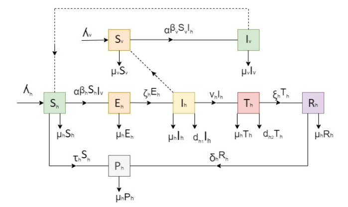
Dengue fever, a vector-borne disease, has affected the whole world in general and the Indian subcontinent in particular for the last three decades. Dengue fever has a significant economic and health impact worldwide; it is essential to develop new mathematical models to study not only the dynamics of the disease but also to suggest cost-effective mechanisms to control disease. In this paper, we design modified facts about the dynamics of this disease more realistically by formulating a new basic $ S_hE_hI_hR_h $ host population and $ S_vI_v $ vector population integer order model, later converting it into a fractional-order model with the help of the well-known Atangana-Baleanu derivative. In this design, we introduce two more compartments, such as the treatment compartment $ T_h $, and the protected traveler compartment $ P_h $ in the host population to produce $ S_hE_hI_hT_hR_hP_h $. We present some observational results by investigating the model for the existence of a unique solution as well as by proving the positivity and boundedness of the solution. We compute reproduction number $ \mathcal{R}_{0} $ by using a next-generation matrix method to estimate the contagious behavior of the infected humans by the disease. In addition, we prove that disease free and endemic equilibrium points are locally and globally stable with restriction to reproduction number $ \mathcal{R}_{0} $. The second goal of this article is to formulate an optimal control problem to study the effect of the control strategy. We implement the Toufik-Atangana scheme for the first time to solve both of the state and adjoint fractional differential equations with the ABC derivative operator. The numerical results show that the fractional order and the different constant treatment rates affect the dynamics of the disease. With an increase in the fractional order and the treatment rate, exposed and infected humans, as well as the infected mosquitoes, decrease. However, the optimal control analysis reveals that the implemented optimal control strategy is very effective for disease control.

| [1] |
D. W. Vaughn, S. Green, S. Kalayanarooj, B. L. Innis, S. Nimmannitya, S. Suntayakorn, et al., Dengue viremia titer, antibody response pattern, and virus serotype correlate with disease severity, J. Infect. Dis., 181 (2000), 2–9. http://doi.org/10.1086/315215 doi: 10.1086/315215

|
| [2] |
C. Li, Y. Lu, J. Liu, X. Wu, Climate change and dengue fever transmission in China: Evidences and challenges, Sci. Total Environ., 622–623 (2018), 493–501. http://doi.org/ 10.1016/j.scitotenv.2017.11.326 doi: 10.1016/j.scitotenv.2017.11.326
|
| [3] | A. Abidemi, N. A. B. Aziz, Analysis of deterministic models for dengue disease transmission dynamics with vaccination perspective in Johor, Malaysia, Int. J. Appl. Comput. Math., 8 (2022). https://doi.org/10.1007/s40819-022-01250-3 |
| [4] | A. Dwivedi, R. Keval, Analysis for transmission of dengue disease with different class of human population, Epidemiol. Method., 10 (2021). https://doi.org/10.1515/em-2020-0046 |
| [5] | E. Soewono, A. K. Supriatna, A two-dimensional model for the transmission of dengue fever disease, B. Malays. Math. Sci. So., 24 (2001), 49–57. |
| [6] | A. Abidemi, H. O. Fatoyinbo, J. K. K. Asamoah, Analysis of dengue fever transmission dynamics with multiple controls: A mathematical approach, In: 2020 International Conference on Decision Aid Sciences and Application (DASA), Sakheer, Bahrain, 2020,971–978. https://doi.org/10.1109/DASA51403.2020.9317064 |
| [7] | P. Pongsumpun, Mathematical model of dengue disease with the incubation period of virus, World Aca. Sci. Eng. Tech., 44 (2009), 328–332. |
| [8] | S. T. R. Pinho, C. P. Ferreira, L. Esteva, F. R. Barreto, V. M. Silva, M. G. L. Teixeira, Modelling the dynamics of dengue real epidemics, Philos. T. Roy. Soc. Math. Phys. Eng. Sci., 368 (2010). https://doi.org/10.1098/rsta.2010.0278 |
| [9] | R. Kongnuy, P. Pongsumpun, Mathematical modeling for dengue transmission with the effect of season, Int. J. Biol. Med. Sci., 7 (2011). |
| [10] | S. Side, S. M. Noorani, A SIR model for spread of dengue fever disease (simulation for South Sulawesi, Indonesia and Selangor, Malaysia), World J. Model. Simul., 9 (2013), 96–105. |
| [11] |
S. Gakkhar, N. C. Chavda, Impact of awareness on the spread of dengue infection in human population, Appl. Math., 4 (2013), 142–147. http://dx.doi.org/10.4236/am.2013.48A020 doi: 10.4236/am.2013.48A020
|
| [12] |
E. Bonyah, M. A. Khan, K. O. Okosun, J. F. Gómez-Aguilar, On the co-infection of dengue fever and Zika virus, Optim. Control Appl. Method., 40 (2019), 394–421. https://doi.org/10.1002/oca.2483 doi: 10.1002/oca.2483
|
| [13] | J. K. K. Asamoah, E. Yankson, E. Okyere, G. Q. Sun, Z. Jin, R. Jan, et al., Optimal control and cost-effectiveness analysis for dengue fever model with asymptomatic and partial immune individuals, Results Phys., 31 (2021). https://doi.org/10.1016/j.rinp.2021.104919 |
| [14] |
R. Jan, S. Boulaaras, Analysis of fractional order dynamics of dengue infection with non-linear incidence functions, T. I. Meas. Control, 44 (2022), 2630–2641. https://doi.org/10.1177/01423312221085049 doi: 10.1177/01423312221085049
|
| [15] | R. Jan, S. Boulaaras, S. Alyobi, K. Rajagopal, M. Jawad, Fractional dynamics of the transmission phenomena of dengue infection with vaccination, Discrete Cont. Dyn. Syst.-S, 2022. https://doi.org/10.3934/dcdss.2022154 |
| [16] | K. Diethelm, The analysis of fractional differential equations: An application-oriented exposition using differential operators of Caputo type, Springer Science and Business Media, Berlin, 2010. |
| [17] | M. Saeedian, M. Khalighi, N. Azimi-Tafreshi, G. Jafari, M. Ausloos, Memory effects on epidemic evolution: The susceptible-infected-recovered epidemic model, Phys. Rev., 95 (2017). https://doi.org/10.1103/PhysRevE.95.022409 |
| [18] |
K. Diethelm, A fractional calculus based model for the simulation of an outbreak of dengue fever, Nonlinear Dynam., 71 (2013), 613–619. https://doi.org/10.1007/s11071-012-0475-2 doi: 10.1007/s11071-012-0475-2
|
| [19] |
M. A. Khan, S. Ullah, M. Farooq, A new fractional model for tuberculosis with relapse via Atangana-Baleanu derivative, Chaos Soliton. Fract., 116 (2018), 227–238. https://doi.org/10.1016/j.chaos.2018.09.039 doi: 10.1016/j.chaos.2018.09.039
|
| [20] |
S. Ullah, M. A. Khan, M. Farooq, A fractional model for the dynamics of tuberculosis virus, Chaos Soliton. Fract., 116 (2018), 63–71. https://doi.org/10.1016/j.chaos.2018.09.001 doi: 10.1016/j.chaos.2018.09.001
|
| [21] |
H. W. Berhe, S. Qureshi, A. A. Shaikh, Deterministic modeling of dysentery diarrhea epidemic under fractional Caputo differential operator via real statistical analysis, Chaos Soliton. Fract., 131 (2020), 109536, https://doi.org/10.1016/j.chaos.2019.109536 doi: 10.1016/j.chaos.2019.109536
|
| [22] |
S. Qureshi, Z. N. Memon, Monotonically decreasing behavior of measles epidemic well captured by Atangana-Baleanu-Caputo fractional operator under real measles data of Pakistan, Chaos Soliton. Fract., 131 (2020), 109478, https://doi.org/10.1016/j.chaos.2019.109478 doi: 10.1016/j.chaos.2019.109478
|
| [23] | S. E. Alhazmi, S. A. M. Abdelmohsen, M. A. Alyami, A. Ali, J. K. K. Asamoah, A novel analysis of generalized perturbed Zakharov-Kuznetsov equation of fractional-order arising in dusty Plasma by natural transform decomposition method, Hindawi J. Nanomater., 2022 (2022). https://doi.org/10.1155/2022/7036825 |
| [24] | L. Zhang, E. Addai, J. Ackora-Prah, Y. D. Arthur, J. K. K. Asamoah, Fractional-order Ebola-Malaria coinfection model with a focus on detection and treatment rate, Hindawi Comput. Math. Method. Med., 2022 (2022). https://doi.org/10.1155/2022/6502598 |
| [25] | R. Alharbi, R. Jan, S. Alyobi, Y. Altayeb, Z. Khan, Mathematical modeling and stability analysis of the dynamics of monkeypox via fractional calculus, Fractals, 30 (2022). https://doi.org/10.1142/S0218348X22402666 |
| [26] |
E. Addai, L. L. Zhang, J. Ackora-Prah, J. F. Gordon, J. K. K. Asamoah, J. F. Essel, Fractal-fractional order dynamics and numerical simulations of a Zika epidemic model with insecticide-treated nets, Physica A, 603 (2022), 127809. https://doi.org/10.1016/j.physa.2022.127809 doi: 10.1016/j.physa.2022.127809
|
| [27] | I. Podlubny, Fractional differential equations: An introduction to fractional derivatives, fractional differential equations, to methods of their solution and some of their applications, Academic Press, Mathematics in Science and Engineering, 1998. |
| [28] |
J. Ackora-Prah, B. Seidu, E. Okyere, J. K. K. Asamoah, Fractal-fractional Caputo maize streak virus disease model, Fractal Fract., 7 (2023), 189. https://doi.org/10.3390/fractalfract7020189 doi: 10.3390/fractalfract7020189
|
| [29] |
M. Caputo, M. Fabrizio, A new definition of fractional derivative without singular kernel, Progr. Fract. Differ. Appl., 1 (2015), 1–13. https://doi.org/10.12785/pfda/010201 doi: 10.12785/pfda/010201
|
| [30] | A. I. K. Butt, M. Imran, S. Batool, M. A. Nuwairan, Theoretical analysis of a COVID-19 CF-fractional model to optimally control the spread of pandemic, Symmetry, 15 (2023). https://doi.org/10.3390/sym15020380 |
| [31] | E. Addai, L. L. Zhang, A. K. Preko, J. K. K. Asamoah, Fractional order epidemiological model of SARS-CoV-2 dynamism involving Alzheimer's disease, Healthcare Anal., 2 (2022). https://doi.org/10.1016/j.health.2022.100114 |
| [32] |
A. Atangana, D. Baleanu, New fractional derivatives with nonlocal and non-singular kernel: Theory and application to heat transfer model, Therm. Sci., 20 (2016), 763–769. https://doi.org/10.2298/TSCI160111018A doi: 10.2298/TSCI160111018A
|
| [33] |
R. Jan, S. Alyobi, M. Inc, A. S. Alshomrani, M. Farooq, A robust study of the transmission dynamics of malaria through non-local and non-singular kernel, AIMS Math., 8 (2023), 7618–7640. https://doi.org/10.3934/math.2023382 doi: 10.3934/math.2023382
|
| [34] | J. K. K. Asamoah, Fractal fractional model and numerical scheme based on Newton polynomial for Q fever disease under Atangana-Baleanu derivative, Results Phys., 34 (2022). https://doi.org/10.1016/j.rinp.2022.105189 |
| [35] | A. A. Kilbas, H. M. Srivastava, J. J. Trujillo, Theory and applications of fractional differential equations, North-Holland Mathematics Studies, 2006. |
| [36] | S. Ullah, M. A. Khan, M. Farooq, E. O. Alzahrani, A fractional model for the dynamics of tuberculosis (TB) using Atangana-Baleanu derivative, Discrete Cont. Dyn. Syst.-S, 13 (2018). https://doi.org/10.3934/dcdss.2020055 |
| [37] |
K. Shah, F. Jarad, T. Abdeljawad, On a nonlinear fractional order model of dengue fever disease under Caputo-Fabrizio derivative, Alex. Eng. J., 59 (2020), 2305–2313. https://doi.org/10.1016/j.aej.2020.02.022 doi: 10.1016/j.aej.2020.02.022
|
| [38] | K. M. Altaf, A. Atangana, Dynamics of Ebola disease in the framework of different fractional derivatives, Entropy, 21 (2019). https://doi.org/10.3390/e21030303 |
| [39] |
J. Losada, J. J. Nieto, Properties of a fractional derivative without singular kernel, Prog. Fract. Diff. Appl., 1 (2015), 87–92. https://doi.org/10.12785/pfda/010202 doi: 10.12785/pfda/010202
|
| [40] | J. K. K. Asamoah, E. Okyere, E. Yankson, A. A. Opoku, A. Adom-Konadu, E. Acheampong, et al., Non-fractional and fractional mathematical analysis and simulations for Q fever, Chaos Soliton. Fract., 156 (2022). https://doi.org/10.1016/j.chaos.2022.111821 |
| [41] | H. Wang, H. Jahanshahi, M. K. Wang, S. Bekiros, J. Liu, A. A. Aly, A Caputo-Fabrizio fractional-order model of HIV/AIDS with a treatment compartment: Sensitivity analysis and optimal control strategies, Entropy, 23 (2021). https://doi.org/10.3390/e23050610 |
| [42] | C. T. Deressa, Y. O. Mussa, G. F. Duressa, Optimal control and sensitivity analysis for transmission dynamics of coronavirus, Results Phys., 19 (2020). https://doi.org/10.1016/j.rinp.2020.103642 |
| [43] |
T. T. Yusuf, F. Benyah, Optimal strategy for controlling the spread of HIV/AIDS disease: A case study of South Africa, J. Biol. Dyn., 6 (2012), 475–494. https://doi.org/10.1080/17513758.2011.628700 doi: 10.1080/17513758.2011.628700
|
| [44] |
E. Bonyah, M. L. Juga, C. W. Chukwu, Fatmawati, A fractional order dangue fever model in the context of protected travelers, Alex. Eng. J., 61 (2022), 927–936. https://doi.org/10.1016/j.aej.2021.04.070 doi: 10.1016/j.aej.2021.04.070
|
| [45] | I. Podlubny, Fractional differential equations: An introduction to fractional derivatives, fractional differential equations, to methods of their solution and some of their applications, Elsevier, 1999. |
| [46] |
D. Baleanu, A. Fernandez, On some new properties of fractional derivatives with Mittag Leffler kernel, Commun. Nonlinear Sci., 59 (2018), 444–462. https://doi.org/10.1016/j.cnsns.2017.12.003 doi: 10.1016/j.cnsns.2017.12.003
|
| [47] |
A. Atangana, I. Koca, Chaos in a simple nonlinear system with Atangana-Baleanu derivative with fractional order, Chaos Soliton. Fract., 89 (2016), 447–454. https://doi.org/10.1016/j.chaos.2016.02.012 doi: 10.1016/j.chaos.2016.02.012
|
| [48] | E. Kreyszig, Introductry functional analysis with application, John Wiley and Sons, New York, 1993. |
| [49] | V. I. Arnold, Ordinary differential equations, MIT Press, London, UK, 1998. |
| [50] | W. Ahmad, M. Abbas, M. Rafiq, D. Baleanu, Mathematical analysis for the effect of voluntary vaccination on the propagation of Corona virus pandemic, Results Phys., 31 (2021), https://doi.org/10.1016/j.rinp.2021.104917 |
| [51] |
W. Ahmad, M. Abbas, Effect of quarantine on transmission dynamics of Ebola virus epidemic: A mathematical analysis, Eur. Phys. J. Plus, 136 (2021), 1–33. https://doi.org/10.1140/epjp/s13360-021-01360-9 doi: 10.1140/epjp/s13360-021-01360-9
|
| [52] |
W. Ahmad, M. Rafiq, M. Abbas, Mathematical analysis to control the spread of Ebola virus epidemic through voluntary vaccination, Eur. Phys. J. Plus, 135 (2020), 1–34. https://doi.org/10.1140/epjp/s13360-020-00683-3 doi: 10.1140/epjp/s13360-020-00683-3
|
| [53] | M. Toufik, A. Atangana, New numerical approximation of fractional derivative with non-local and non-singular kernel: Application to chaotic models, Eur. Phys. J. Plus, 132 (2017). https://doi.org/10.1140/epjp/i2017-11717-0 |
| [54] |
M. A. Khan, A. Atangana, Modeling the dynamics of novel coronavirus (2019-nCov) with fractional derivative, Alex. Eng. J., 59 (2020), 2379–2389. https://doi.org/10.1016/j.aej.2020.02.033 doi: 10.1016/j.aej.2020.02.033
|
| [55] |
R. Kamocki, Pontryagin maximum principle for fractional ordinary optimal control problems, Math. Method. Appl. Sci., 37 (2014), 1668–1686. https://doi.org/10.1002/mma.2928 doi: 10.1002/mma.2928
|
| [56] | S. Lenhart, J. T. Workman, Optimal control applied to biological models, CRC Press, 2007. |
| [57] | H. M. Ali, F. L. Pereira, S. M. Gama, A new approach to the Pontryagin maximum principle for nonlinear fractional optimal control problems, Math. Method. Appl. Sci., 39 (2016). https://doi.org/10.1002/mma.3811 |
| [58] |
C. Vargas-De-Len, Volterra-type Lyapunov functions for fractional-order epidemic systems, Commun. Nonlinear Sci., 24 (2015), 75–85. https://doi.org/10.1016/j.cnsns.2014.12.013 doi: 10.1016/j.cnsns.2014.12.013
|
| [59] | J. P. LaSalle, The stability of dynamical systems, SIAM, Philadelphia, PA, 1976. |


Figures(9) / Tables(2)

Asma Hanif, Azhar Iqbal Kashif Butt. Atangana-Baleanu fractional dynamics of dengue fever with optimal control strategies[J]. AIMS Mathematics, 2023, 8(7): 15499-15535. doi: 10.3934/math.2023791


 DownLoad: