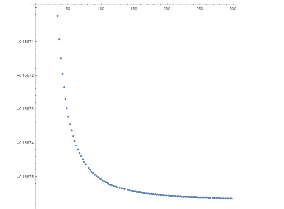
The exterior transmission eigenvalues corresponding to spherical symmetry media and spherically symmetric eigenfunctions are considered. Under various coefficient conditions, we give the number and the asymptotic distribution (described by the subscript numbers) of these eigenvalues in the complex plane.
Citation: Yalin Zhang, Jia Zhao. The distribution of exterior transmission eigenvalues for spherically stratified media[J]. AIMS Mathematics, 2023, 8(4): 9647-9670. doi: 10.3934/math.2023487
The exterior transmission eigenvalues corresponding to spherical symmetry media and spherically symmetric eigenfunctions are considered. Under various coefficient conditions, we give the number and the asymptotic distribution (described by the subscript numbers) of these eigenvalues in the complex plane.

| [1] | F. Cakoni, D. Colton, A qualitative approach to inverse theory, New York: Springer, 2014. http://dx.doi.org/10.1007/978-1-4614-8827-9 |
| [2] |
T. Aktosun, V. Papanicolaou, Transmission eigenvalues for the self-adjoint Schröinger operator on the half line, Inverse Probl., 30 (2014), 075001. http://dx.doi.org/10.1088/0266-5611/30/7/075001 doi: 10.1088/0266-5611/30/7/075001

|
| [3] |
T. Aktosun, D. Gintides, V. Papanicolaou, The uniqueness in the inverse problem for transmission eigenvalues for the spherically symmetric variable-speed wave equation, Inverse Probl., 27 (2011), 115004. http://dx.doi.org/10.1088/0266-5611/27/11/115004 doi: 10.1088/0266-5611/27/11/115004
|
| [4] |
T. Aktosun, V. Papanicolaou, Reconstruction of the wave speed from transmission eigenvalues for the spherically-symmetric variable-speed wave equation, Inverse Probl., 29 (2013), 065007. http://dx.doi.org/10.1088/0266-5611/29/6/065007 doi: 10.1088/0266-5611/29/6/065007
|
| [5] |
N. Bondarenko, S. Buterin, On a local solvability and stability of the inverse transmission eigenvalue problem, Inverse Probl., 33 (2017), 115010. http://dx.doi.org/10.1088/1361-6420/aa8cb5 doi: 10.1088/1361-6420/aa8cb5
|
| [6] |
S. Buterin, C. Yang, V. Yurko, On an open question in the inverse transmission eigenvalue problem, ems, Inverse Probl., 31 (2015), 045003. http://dx.doi.org/10.1088/0266-5611/31/4/045003 doi: 10.1088/0266-5611/31/4/045003
|
| [7] |
S. Buterin, C. Yang, On an inverse transmission problem from complex eigenvalues, Results Math., 71 (2017), 859–866. http://dx.doi.org/10.1007/s00025-015-0512-9 doi: 10.1007/s00025-015-0512-9
|
| [8] |
F. Cakoni, D. Colton, D. Gintides, The interior transmission eigenvalue problem, SIAM J. Math. Anal., 42 (2010), 2912–2921. http://dx.doi.org/10.1137/100793542 doi: 10.1137/100793542
|
| [9] |
D. Colton, Y. Leung, S. Meng, Distribution of complex transmission eigenvalues for spherically stratified media, Inverse Probl., 31 (2015), 035006. http://dx.doi.org/10.1088/0266-5611/31/3/035006 doi: 10.1088/0266-5611/31/3/035006
|
| [10] |
D. Colton, Y. Leung, The existence of complex transmission eigenvalues for spherically stratified media, Appl. Anal., 96 (2017), 39–47. http://dx.doi.org/10.1080/00036811.2016.1210788 doi: 10.1080/00036811.2016.1210788
|
| [11] |
L. Chen, On the inverse spectral theory in a non-homogeneous interior transmission problem, Complex Var. Elliptic, 60 (2015), 707–731. http://dx.doi.org/10.1080/17476933.2014.970541 doi: 10.1080/17476933.2014.970541
|
| [12] |
J. McLaughlin, P. Polyakov, On the uniqueness of a spherically symmetric speed of sound from transmission eigenvlaues, J. Differ. Equations, 107 (1994), 351–382. http://dx.doi.org/10.1006/jdeq.1994.1017 doi: 10.1006/jdeq.1994.1017
|
| [13] |
G. Wei, H. Xu, Inverse spectral analysis for the transmission eigenvalue problem, Inverse Probl., 29 (2013), 115012. http://dx.doi.org/10.1088/0266-5611/29/11/115012 doi: 10.1088/0266-5611/29/11/115012
|
| [14] |
X. Xu, X. Xu, C. Yang, Distribution of transmission eigenvalues and inverse spectral analysis with partial information on the refractive index, Math. Method. Appl. Sci., 39 (2016), 5330–5342. http://dx.doi.org/10.1002/mma.3918 doi: 10.1002/mma.3918
|
| [15] |
Y. Zhang, Spectral properties of exterior transmission problem for spherically stratified anisotropic media, Appl. Anal., 100 (2021), 1668–1692. http://dx.doi.org/10.1080/00036811.2019.1659956 doi: 10.1080/00036811.2019.1659956
|
| [16] |
Y. Zhang, G. Shi, The uniqueness for inverse discrete exterior transmission eigenvalue problems in spherically symmetric media, Appl. Anal., 100 (2021), 3463–3477. http://dx.doi.org/10.1080/00036811.2020.1721474 doi: 10.1080/00036811.2020.1721474
|
| [17] |
S. Buterin, A. Choque-Rivero, M. Kuznetsova, On a regularization approach to the inverse transmission eigenvalue problem, Inverse Probl., 36 (2020), 105002. http://dx.doi.org/10.1088/1361-6420/abaf3c doi: 10.1088/1361-6420/abaf3c
|
| [18] |
P. Jakubik, R. Potthast, Testing the integrity of some cavity-the Cauchy problem and the range test, Appl. Numer. Math., 58 (2008), 899–914. http://dx.doi.org/10.1016/j.apnum.2007.04.007 doi: 10.1016/j.apnum.2007.04.007
|
| [19] |
D. Colton, S. Meng, Spectral properties of the exterior transmission eigenvalue problem, Inverse Probl., 30 (2014), 105010. http://dx.doi.org/10.1088/0266-5611/30/10/105010 doi: 10.1088/0266-5611/30/10/105010
|
| [20] |
S. Meng, H. Haddar, F. Cakoni, The factorization method for a cavity in an inhomogeneous medium, Inverse Probl., 30 (2014), 045008. http://dx.doi.org/10.1088/0266-5611/30/4/045008 doi: 10.1088/0266-5611/30/4/045008
|
| [21] |
F. Cakoni, D. Colton, P. Monk, On the use of transmission eigenvalues to estimate the index of refraction from far field data, Inverse Probl., 23 (2007), 507. http://dx.doi.org/10.1088/0266-5611/23/2/004 doi: 10.1088/0266-5611/23/2/004
|
| [22] |
F. Cakoni, M. Cayoren, D. Colton, Transmission eigenvalues and the nondestructive testing of dielectrics, Inverse Probl., 24 (2008), 065016. http://dx.doi.org/10.1088/0266-5611/24/6/065016 doi: 10.1088/0266-5611/24/6/065016
|
| [23] |
X. Xu, C. Yang, S. Buterin, V. Yurko, Estimates of complex eigenvalues and an inverse spectral problem for the transmission eigenvalue problem, Electron. J. Qual. Theory Differ. Equ., 2019 (2019), 1–15. http://dx.doi.org/10.14232/ejqtde.2019.1.38 doi: 10.14232/ejqtde.2019.1.38
|
| [24] |
X. Xu, On the direct and inverse transmission eigenvalue problems for the Schrödinger operator on the half line, Math. Method. Appl. Sci., 43 (2020), 8434–8448. http://dx.doi.org/10.1002/mma.6496 doi: 10.1002/mma.6496
|
| [25] |
L. Chen, An inverse spectral uniqueness in exterior transmission problem, Tsukuba J. Math., 41 (2017), 297–312. http://dx.doi.org/10.21099/tkbjm/1521597627 doi: 10.21099/tkbjm/1521597627
|
| [26] |
E. Blåsten, H. Liu, Scattering by curvatures, radiationless sources, transmission eigenfunctions and inverse scattering problems, SIAM J. Math. Anal., 53 (2021), 3801–3837. http://dx.doi.org/10.1137/20M1384002 doi: 10.1137/20M1384002
|
| [27] |
E. Blåsten, H. Liu, On vanishing near corners of transmission eigenfunctions, J. Funct. Anal., 273 (2017), 3616–3632. http://dx.doi.org/10.1016/j.jfa.2017.08.023 doi: 10.1016/j.jfa.2017.08.023
|
| [28] |
Y. Deng, C. Duan, H. Liu, On vanishing near corners of conductive transmission eigenfunctions, Res. Math. Sci., 9 (2022), 2. https://dx.doi.org/10.1007/s40687-021-00299-8 doi: 10.1007/s40687-021-00299-8
|
| [29] |
H. Diao, X. Cao, H. Liu, On the geometric structures of transmission eigenfunctions with a conductive boundary condition and applications, Commun. Part, Diff, Eq., 46 (2021), 630–679. http://dx.doi.org/10.1080/03605302.2020.1857397 doi: 10.1080/03605302.2020.1857397
|
| [30] |
H. Diao, H. Liu, B. Sun, On a local geometric property of the generalized elastic transmission eigenfunctions and application, Inverse Probl., 37 (2021), 105015. http://dx.doi.org/10.1088/1361-6420/ac23c2 doi: 10.1088/1361-6420/ac23c2
|
| [31] |
H. Diao, H. Liu, X. Wang, K. Yang, On vanishing and localizing around corners of electromagnetic transmission resonance, Partial Differ. Equ. Appl., 2 (2021), 78. http://dx.doi.org/10.1007/s42985-021-00131-6 doi: 10.1007/s42985-021-00131-6
|
| [32] |
Y. Chow, Y. Deng, Y. He, H. Liu, X. Wang, Surface-localized transmission eigenstates, super resolution imaging and pseudo surface plasmon modes, SIAM J. Imaging Sci., 14 (2021), 946–975. http://dx.doi.org/10.1137/20M1388498 doi: 10.1137/20M1388498
|
| [33] |
Y. Deng, Y. Jiang, H. Liu, K. Zhang, On new surface-localized transmission eigenmodes, Inverse Probl. Imag., 16 (2022), 596–611. http://dx.doi.org/10.3934/ipi.2021063 doi: 10.3934/ipi.2021063
|
| [34] |
Y. Deng, H. Liu, X. Wang, W. Wu, On geometrical properties of electromagnetic transmission eigenfunctions and artificial mirage, SIAM J. Appl. Math., 82 (2022), 1–24. http://dx.doi.org/10.1137/21M1413547 doi: 10.1137/21M1413547
|
| [35] | Y. Jiang, H. Liu, J. Zhang, K. Zhang, Boundary localization of transmission eigenfunctions in spherically stratified media, Asymptotic Anal., in press. http://dx.doi.org/10.3233/ASY-221794 |
| [36] |
Y. Wang, C. Shieh, The inverse interior transmission eigenvalue problem with mixed spectral data, Appl. Math. Comput., 343 (2019), 285–298. http://dx.doi.org/10.1016/j.amc.2018.09.014 doi: 10.1016/j.amc.2018.09.014
|
| [37] |
C. Yang, S. Buterin, Uniqueness of the interior transmission problem with partial information on the potential and eigenvalues, J. Differ. Equations, 260 (2016), 4871–4887. http://dx.doi.org/10.1016/j.jde.2015.11.031 doi: 10.1016/j.jde.2015.11.031
|
| [38] |
X. Xu, L. Ma, C. Yang, On the stability of the inverse transmission eigenvalue problem from the data of McLaughlin and Polyakov, J. Differ. Equations, 316 (2022), 222–248. http://dx.doi.org/10.1016/j.jde.2022.01.052 doi: 10.1016/j.jde.2022.01.052
|
| [39] | J. Poschel, E. Trubowitz, Inverse spectral theory, New York: Academic Press, 1987. |
| [40] | B. Levin, Lectures on Entire functions, Providence: American Mathematical Society, 1996. |
Figures(1)

Yalin Zhang, Jia Zhao. The distribution of exterior transmission eigenvalues for spherically stratified media[J]. AIMS Mathematics, 2023, 8(4): 9647-9670. doi: 10.3934/math.2023487


 DownLoad: