Image restoration by using a modified proximal point algorithm

Areerat Arunchai; Thidaporn Seangwattana; Kanokwan Sitthithakerngkiet; Kamonrat Sombut; Areerat Arunchai; Thidaporn Seangwattana; Kanokwan Sitthithakerngkiet; Kamonrat Sombut

doi:10.3934/math.2023482

AIMS Mathematics

2023, Volume 8, Issue 4: 9557-9575. doi: 10.3934/math.2023482

Previous Article Next Article

Research article Special Issues

Image restoration by using a modified proximal point algorithm

1.
Department of Mathematics and Statistics, Faculty of Science and Technology, Nakhon Sawan Rajabhat University, 60000, Nakhon Sawan, Thailand
2.
Faculty of Science Energy and Environment, King Mongkut's University of Technology North Bangkok, Rayong Campus (KMUTNB), 21120, Rayong, Thailand
3.
Intelligent and Nonlinear Dynamic Innovations Research Center, Department of Mathematics Faculty of Applied Science, King Mongkut's University of Technology North Bangkok (KMUTNB), 10800, Bangkok, Thailand
4.
Department of Mathematics and Computer Science, Faculty of Science and Technology, Rajamangala University of Technology Thanyaburi (RMUTT), 12110, Pathum Thani, Thailand
5.
Applied Mathematics for Science and Engineering Research Unit (AMSERU), Department of Mathematics and Computer Science, Faculty of Science and Technology, Rajamangala University of Technology Thanyaburi (RMUTT), 12110, Rungsit-Nakorn Nayok Rd., Klong 6, Khlong Luang, Thanyaburi, Pathum thani, Thailand

Received: 20 September 2022 Revised: 13 February 2023 Accepted: 14 February 2023 Published: 20 February 2023
MSC : 37N40, 49J40

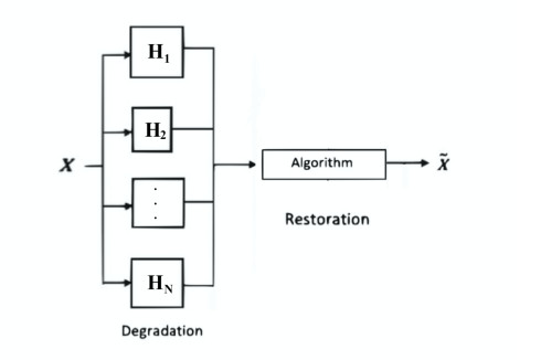
In this paper, we establish a modified proximal point algorithm for solving the common problem between convex constrained minimization and modified variational inclusion problems. The proposed algorithm base on the proximal point algorithm in ^[19] and the method of Khuangsatung and Kangtunyakarn in ^[21] by using suitable conditions in Hilbert spaces. The proposed algorithm is not only presented in this article; however has also been demonstrated to generate a robust convergence theorem. The proposed algorithm could be used to solve image restoration problems where the images have suffered a variety of blurring operations. Additionally, we contrast the signal-to-noise ratio (SNR) of the proposed algorithm against that of Khuangsatung and Kangtunyakarn's method in ^[21] in order to compare image quality.
- convex minimization,
- image restoration,
- optimization,
- proximal point algorithm,
- variational inclusion problem
Citation: Areerat Arunchai, Thidaporn Seangwattana, Kanokwan Sitthithakerngkiet, Kamonrat Sombut. Image restoration by using a modified proximal point algorithm[J]. AIMS Mathematics, 2023, 8(4): 9557-9575. doi: 10.3934/math.2023482

Related Papers:

Abstract

In this paper, we establish a modified proximal point algorithm for solving the common problem between convex constrained minimization and modified variational inclusion problems. The proposed algorithm base on the proximal point algorithm in ^[19] and the method of Khuangsatung and Kangtunyakarn in ^[21] by using suitable conditions in Hilbert spaces. The proposed algorithm is not only presented in this article; however has also been demonstrated to generate a robust convergence theorem. The proposed algorithm could be used to solve image restoration problems where the images have suffered a variety of blurring operations. Additionally, we contrast the signal-to-noise ratio (SNR) of the proposed algorithm against that of Khuangsatung and Kangtunyakarn's method in ^[21] in order to compare image quality.

References

[1]	G. P. Crespi, A. Guerraggio, M. Rocca, Minty variational inequality and optimization: Scalar and vector case, In: Generalized convexity and monotonicity and applications, Boston: Springer, 2005. https://doi.org/10.1007/0-387-23639-2_12
[2]	B. Martinet, Régularisation d'inéquations variationnelles par approximations successives, Recherche Opérationnelle, 4 (1970), 154–158.
[3]	R. T. Rockafellar, Monotone operators and the proximal point algorithm, SIAM J. Control Optim., 14 (1976), 877–898. https://doi.org/10.1137/0314056 doi: 10.1137/0314056
[4]	O. Güler, On the convergence of the proximal point algorithm for convex minimization, SIAM J. Control Optim., 29 (1991), 403–419. https://doi.org/10.1137/032902 doi: 10.1137/032902
[5]	S. Kamimura, W. Takahashi, Strong convergence of a proximal-type algorithm in a Banach space, SIAM J. Optim., 13 (2003), 938–945. https://doi.org/10.1137/S105262340139611X doi: 10.1137/S105262340139611X
[6]	N. Lehdili, A. Moudafi, Combining the proximal algorithm and Tikhonov regularization, Optimization, 37 (1996), 239–252. https://doi.org/10.1080/02331939608844217 doi: 10.1080/02331939608844217
[7]	S. Reich, Strong convergence theorems for resolvents of accretive operators in Banach spaces, J. Math. Anal. Appl., 75 (1980), 287–292. https://doi.org/10.1016/0022-247X(80)90323-6 doi: 10.1016/0022-247X(80)90323-6
[8]	M. V. Solodov, B. F. Svaiter, Forcing strong convergence of proximal point iterations in a Hilbert space, Math. Program., 87 (2000), 189–202. https://doi.org/10.1007/s101079900113 doi: 10.1007/s101079900113
[9]	H. K. Xu, A regularization method for the proximal point algorithm, J. Glob. Optim., 36 (2006), 115–125. https://doi.org/10.1007/s10898-006-9002-7 doi: 10.1007/s10898-006-9002-7
[10]	J. M. Borwein, A. S. Lewis, Convex analysis and nonlinear optimization: Theory and examples, New York: Springer, 2005. https://doi.org/10.1007/978-0-387-31256-9
[11]	T. Seangwattana, K. Sombut, A. Arunchai, K. Sitthithakerngkiet, A modified Tseng's method for solving the modified variational inclusion problems and its applications, Symmetry, 13 (2021), 2250. https://doi.org/10.3390/sym13122250 doi: 10.3390/sym13122250
[12]	P. L. Lions, B. Mercier, Splitting algorithms for the sum of two nonlinear operators, SIAM J. Numer. Anal., 16 (1979), 964–979. https://doi.org/10.1137/0716071 doi: 10.1137/0716071
[13]	G. B. Passty, Ergodic convergence to a zero of the sum of monotone operators in Hilbert spaces, J. Math. Anal. Appl., 72 (1979), 383–390. https://doi.org/10.1016/0022-247X(79)90234-8 doi: 10.1016/0022-247X(79)90234-8
[14]	P. Tseng, A modified forward-backward splitting method for maximal monotone mappings, SIAM J. Control Optim., 38 (1998), 431–446. https://doi.org/10.1137/S0363012998338806 doi: 10.1137/S0363012998338806
[15]	G. H-G. Chen, R. T. Rockafellar, Convergence rates in forward-backward splitting, SIAM J. Optim., 7 (1997), 421–444. https://doi.org/10.1137/S1052623495290179 doi: 10.1137/S1052623495290179
[16]	S. Kamimura, W. Takahashi, Approximating solutions of maximal monotone operators in Hilbert spaces, J. Approx. Theory, 106 (2000), 226–240. https://doi.org/10.1006/jath.2000.3493 doi: 10.1006/jath.2000.3493
[17]	A. Adamu, D. Kitkuan, P. Kumam, A. Padcharoen, T. Seangwattana, Approximation method for monotone inclusion problems in real Banach spaces with applications, J. Inequal. Appl., 70 (2022), 70. https://doi.org/10.1186/s13660-022-02805-0 doi: 10.1186/s13660-022-02805-0
[18]	O. A. Boikanyo, The viscosity approximation forward-backward splitting method for zeros of the sum of monotone operators, Abstr. Appl. Anal., 2016 (2016), 2371857. https://doi.org/10.1155/2016/2371857 doi: 10.1155/2016/2371857
[19]	T. M. M. Sow, A modified proximal point algorithm for solving variational inclusion problem in real Hilbert spaces, e-J. Anal. Appl. Math., 2020 (2020), 28–39. https://doi.org/10.2478/ejaam-2020-0003 doi: 10.2478/ejaam-2020-0003
[20]	W. Khuangsatung, A. Kangtunyakarn, Algorithm of a new variational inclusion problems and strictly pseudononspreading mapping with application, Fixed Point Theory Appl., 2014 (2014), 209. https://doi.org/10.1186/1687-1812-2014-209 doi: 10.1186/1687-1812-2014-209
[21]	W. Khuangsatung, A. Kangtunyakarn, A theorem of variational inclusion problems and various nonlinear mappings, Appl. Anal., 97 (2017), 1172–1186. https://doi.org/10.1080/00036811.2017.1307965 doi: 10.1080/00036811.2017.1307965
[22]	T. M. M. Sow, An iterative algorithm for solving equilibrium problems, variational inequalities and fixed point problems of multivalued quasi-nonexpansive mappings, Appl. Set-Valued Anal. Optim., 1 (2019), 171–185. https://doi.org/10.23952/asvao.1.2019.2.06 doi: 10.23952/asvao.1.2019.2.06
[23]	L. Ambrosio, N. Gigli, G. Savaré, Gradient flows: In metric spaces and in the space of probability measures, Basel: Birkhäuser, 2005. https://doi.org/10.1007/b137080
[24]	J. Jost, Convex functionals and generalized harmonic maps into spaces of nonpositive curvature, Comment. Math. Helvetici, 70 (1995), 659–673. https://doi.org/10.1007/BF02566027 doi: 10.1007/BF02566027
[25]	I. Miyadera, Translations of mathematical monographs: Nonlinear semigroups, Rhode Island: American Mathematical Society, 1992. https://doi.org/10.1090/mmono/109
[26]	S. S. Chang, Y. K. Tang, L. Wang, Y. G. Xu, Y. H. Zhao, G. Wang, Convergence theorems for some multi-valued generalized nonexpansive mappings, Fixed Point Theory Appl., 2014 (2014), 33. https://doi.org/10.1186/1687-1812-2014-33 doi: 10.1186/1687-1812-2014-33
[27]	W. Takahashi, Nonlinear function analysis, Yokohama: Yokohama Publishers, 2000.
[28]	H. K. Xu, Inequalities in Banach spaces with applications, Nonlinear Anal., 16 (1991), 1127–1138. https://doi.org/10.1016/0362-546X(91)90200-K doi: 10.1016/0362-546X(91)90200-K

Reader Comments

Your name:*

Email:*
© 2023 the Author(s), licensee AIMS Press. This is an open access article distributed under the terms of the Creative Commons Attribution License (http://creativecommons.org/licenses/by/4.0)