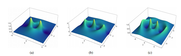
This paper investigates rational solutions of an extended Camassa-Holm-Kadomtsev-Petviashvili equation, which simulates dispersion's role in the development of patterns in a liquid drop, and describes left and right traveling waves like the Boussinesq equation. Through its bilinear form and symbolic computation, we derive some multiple order rational and generalized rational solutions and analyze their dynamic features, such as the connection between rational solution and bilinear equation, scatter behavior, moving path, and exact location of the soliton. The obtained solutions demonstrate two wave forms: multi-lump and multi-wave that consist of three, six and eight lump waves or two, three and four line waves. Moreover, different from the multi-wave solitons, stationary multiple dark waves are presented.
Citation: Zhe Ji, Yifan Nie, Lingfei Li, Yingying Xie, Mancang Wang. Rational solutions of an extended (2+1)-dimensional Camassa-Holm- Kadomtsev-Petviashvili equation in liquid drop[J]. AIMS Mathematics, 2023, 8(2): 3163-3184. doi: 10.3934/math.2023162
This paper investigates rational solutions of an extended Camassa-Holm-Kadomtsev-Petviashvili equation, which simulates dispersion's role in the development of patterns in a liquid drop, and describes left and right traveling waves like the Boussinesq equation. Through its bilinear form and symbolic computation, we derive some multiple order rational and generalized rational solutions and analyze their dynamic features, such as the connection between rational solution and bilinear equation, scatter behavior, moving path, and exact location of the soliton. The obtained solutions demonstrate two wave forms: multi-lump and multi-wave that consist of three, six and eight lump waves or two, three and four line waves. Moreover, different from the multi-wave solitons, stationary multiple dark waves are presented.

| [1] |
L. Draper, 'Freak' ocean waves, Weather, 21 (1966), 2–4. https://doi.org/10.1002/j.1477-8696.1966.tb05176.x doi: 10.1002/j.1477-8696.1966.tb05176.x

|
| [2] |
P. Muller, C. Garrett, A. Osborne, Rogue waves, Oceanography, 18 (2005), 66–75. http://dx.doi.org/10.5670/oceanog.2005.30 doi: 10.5670/oceanog.2005.30
|
| [3] |
V. E. Zakharov, Stability of periodic waves of finite amplitude on the surface of a deep fluid, J. Appl. Mech. Tech. Phys., 9 (1968), 190–194. https://doi.org/10.1007/BF00913182 doi: 10.1007/BF00913182
|
| [4] |
A. Ankiewicz, N. Devine, N. Akhmediev, Are rogue waves robust against perturbations?, Phys. Lett. A, 373 (2009), 3997–4000. https://doi.org/10.1016/j.physleta.2009.08.053 doi: 10.1016/j.physleta.2009.08.053
|
| [5] |
N. Akhmediev, J. M. Soto-Crespo, A. Ankiewicz, Extreme waves that appear from nowhere: on the nature of rogue waves, Phys. Lett. A, 373 (2009), 2137–2145. https://doi.org/10.1016/j.physleta.2009.04.023 doi: 10.1016/j.physleta.2009.04.023
|
| [6] |
T. B. Benjamin, J. E. Feir, The disintegration of wave trains on deep water Part 1. Theory, J. Fluid. Mech., 27 (1967), 417–430. https://doi.org/10.1017/S002211206700045X doi: 10.1017/S002211206700045X
|
| [7] |
A. M. Turing, The chemical basis of morphogenesis, Bltn. Mathcal. Biology, 52 (1990), 153–197. https://doi.org/10.1007/BF02459572 doi: 10.1007/BF02459572
|
| [8] |
N. Akhmediev, A. Ankiewicz, J. M. Soto-Crespo, Rogue waves and rational solutions of the nonlinear Schrrödinger equation, Phys. Rev. E, 80 (2009), 026601. https://doi.org/10.1103/PhysRevE.80.026601 doi: 10.1103/PhysRevE.80.026601
|
| [9] |
W. X. Ma, Lump solutions to the Kadomtsev-Petviashvili equation, Phys. Lett. A, 379 (2015), 1975–1978. https://doi.org/10.1016/j.physleta.2015.06.061 doi: 10.1016/j.physleta.2015.06.061
|
| [10] |
S. F. Tian, D. Guo, X. B. Wang, T. T. Zhang, Traveling wave, lump wave, rogue wave, multi-kink solitary wave and interaction solutions in a (3+1)-dimensional Kadomtsev-Petviashvili equation with Bäcklund transformation, J. Appl. Anal. Comput., 11 (2021), 45–58. https://doi.org/10.11948/20190086 doi: 10.11948/20190086
|
| [11] |
Z. Y. Yin, S. F. Tian, Nonlinear wave transitions and their mechanisms of (2+1)-dimensional Sawada-Kotera equation, Physica D, 427 (2021), 133002. https://doi.org/10.1016/j.physd.2021.133002 doi: 10.1016/j.physd.2021.133002
|
| [12] |
Z. Y. Wang, S. F. Tian, J. Cheng, The $\bar{\partial}$-dressing method and soliton solutions for the three-component coupled Hirota equations, J. Math. Phys., 62 (2021), 093510. https://doi.org/10.1063/5.0046806 doi: 10.1063/5.0046806
|
| [13] |
X. Wang, L. Wang, C. Liu, B. W. Guo, J. Wei, Rogue waves, semirational rogue waves and W-shaped solitons in the three-level coupled Maxwell-Bloch equations, Commun. Nonlinear Sci., 107 (2022), 106172. https://doi.org/10.1016/j.cnsns.2021.106172 doi: 10.1016/j.cnsns.2021.106172
|
| [14] |
X. Wang, L. Wang, J. Wei, B. W. Guo, J. F. Kang, Rogue waves in the three-level defocusing coupled Maxwell-Bloch equations, Proc. R. Soc. A, 477 (2021), 20210585. https://doi.org/10.1098/rspa.2021.0585 doi: 10.1098/rspa.2021.0585
|
| [15] |
J. C. Chen, Z. Y. Ma, Y. H. Hu, Nonlocal symmetry, Darboux transformation and soliton-cnoidal wave interaction solution for the shallow water wave equation, J. Math. Anal. Appl., 460 (2018), 987–1003. https://doi.org/10.1016/j.jmaa.2017.12.028 doi: 10.1016/j.jmaa.2017.12.028
|
| [16] |
X. Wang, J. Wei, Three types of Darboux transformation and general soliton solutions for the space-shifted nonlocal PT symmetric nonlinear Schrödinger equation, Appl. Math. Lett., 130 (2022), 107998. https://doi.org/10.1016/j.aml.2022.107998 doi: 10.1016/j.aml.2022.107998
|
| [17] |
J. C. Chen, Z. Y. Ma, Consistent Riccati expansion solvability and soliton-cnoidal wave interaction solution of a (2+1)-dimensional Korteweg-de Vries equation, Appl. Math. Lett., 64 (2017), 87–93. https://doi.org/10.1016/j.aml.2016.08.016 doi: 10.1016/j.aml.2016.08.016
|
| [18] |
J. C. Chen, S. D. Zhu, Residual symmetries and soliton-cnoidal wave interaction solutions for the negative-order Korteweg-de Vries equation, Appl. Math. Lett., 73 (2017), 136–142. https://doi.org/10.1016/j.aml.2017.05.002 doi: 10.1016/j.aml.2017.05.002
|
| [19] |
X. Y. Gao, Y. J. Guo, W. R. Shan, Optical waves/modes in a multicomponent inhomogeneous optical fiber via a three-coupled variable-coefficient nonlinear Schrödinger system, Appl. Math. Lett., 120 (2021), 107161. https://doi.org/10.1016/j.aml.2021.107161 doi: 10.1016/j.aml.2021.107161
|
| [20] |
X. Y. Gao, Y. J. Guo, W. R. Shan, Taking into consideration an extended coupled (2+1)-dimensional Burgers system in oceanography, acoustics and hydrodynamics, Chaos Soliton. Fract., 161 (2022), 112293. https://doi.org/10.1016/j.chaos.2022.112293 doi: 10.1016/j.chaos.2022.112293
|
| [21] |
X. Y. Gao, Y. J. Guo, W. R. Shan, Similarity reductions for a generalized (3+1)-dimensional variable-coefficient B-type Kadomtsev-Petviashvili equation in fluid dynamics, Chinese J. Phys., 77 (2022), 2707–2712. https://doi.org/10.1016/j.cjph.2022.04.014 doi: 10.1016/j.cjph.2022.04.014
|
| [22] |
X. Y. Gao, Y. J. Guo, W. R. Shan, T. Y. Zhou, M. Wang, D. Y. Yang, In the atmosphere and oceanic fluids: scaling transformations, bilinear forms, Bäcklund transformations and solitons for a generalized variable-coefficient Korteweg-de Vries-modified Korteweg-de Vries equation, China Ocean Eng., 35 (2021), 518–530. https://doi.org/10.1007/s13344-021-0047-7 doi: 10.1007/s13344-021-0047-7
|
| [23] |
X. Y. Gao, Y. J. Guo, W. R. Shan, D. Y. Yang, Bilinear forms through the binary Bell polynomials, N solitons and Bäcklund transformations of the Boussinesq-Burgers system for the shallow water waves in a lake or near an ocean beach, Commun. Theor. Phys., 72 (2020), 095002. https://doi.org/10.1088/1572-9494/aba23d doi: 10.1088/1572-9494/aba23d
|
| [24] |
X. Y. Gao, Y. J. Guo, W. R. Shan, D. Y. Yang, Regarding the shallow water in an ocean via a Whitham-Broer-Kaup-like system: hetero-Bäcklund transformations, bilinear forms and M solitons, Chaos Soliton. Fract., 162 (2022), 112486. https://doi.org/10.1016/j.chaos.2022.112486 doi: 10.1016/j.chaos.2022.112486
|
| [25] |
R. Camassa, D. D. Holm, An integrable shallow water equation with peaked solitons, Phys. Rev. Lett., 71 (1993), 1661–1664. https://doi.org/10.1103/PhysRevLett.71.1661 doi: 10.1103/PhysRevLett.71.1661
|
| [26] |
Y. Zhang, H. Dong, X. Zhang, H. Yang, Rational solutions and lump solutions to the generalized (3+1)-dimensional shallow water-like equation, Comput. Math. Appl., 73 (2017), 246–252. https://doi.org/10.1016/j.camwa.2016.11.009 doi: 10.1016/j.camwa.2016.11.009
|
| [27] |
T. B. Benjamin, J. L. Bona, J. J. Mahony, Model equations for long waves in nonlinear dispersive systems, Phil. Trans. R. Soc. A, 272 (1972), 47–78. https://doi.org/10.1098/rsta.1972.0032 doi: 10.1098/rsta.1972.0032
|
| [28] |
A. Mekki, M. M. Ali, Numerical simulation of Kadomtsev-Petviashvili-Benjamin-Bona-Mahony equations using finite difference method, Appl. Math. Comput., 219 (2013), 11214–11222. https://doi.org/10.1016/j.amc.2013.04.039 doi: 10.1016/j.amc.2013.04.039
|
| [29] |
Y. Yin, B. Tian, X. Y. Wu, H. M. Yin, C. R. Zhang, Lump waves and breather waves for a (3+1)-dimensional generalized Kadomtsev-Petviashvili Benjamin-Bona-Mahony equation for an offshore structure, Mod. Phys. Lett. B, 32 (2018), 1850031. https://doi.org/10.1142/S0217984918500318 doi: 10.1142/S0217984918500318
|
| [30] |
D. J. Korteweg, G. de Vries, On the change of form of long waves advancing in a rectangular canal, and on a new type of long stationary waves, The London, Edinburgh, and Dublin Philosophical Magazine and Journal of Science, 39 (1895), 422–443. https://doi.org/10.1080/14786449508620739 doi: 10.1080/14786449508620739
|
| [31] |
Z. Liu, R. Wang, Z. Jing, Peaked wave solutions of Camassa-Holm equation, Chaos Soliton. Fract., 19 (2004), 77–92. https://doi.org/10.1016/S0960-0779(03)00082-1 doi: 10.1016/S0960-0779(03)00082-1
|
| [32] |
W. Liu, Y. Zhang, Families of exact solutions of the generalized (3+1)-dimensional nonlinear-wave equation, Mod. Phys. Lett. B, 32 (2018), 1850359. https://doi.org/10.1142/S0217984918503591 doi: 10.1142/S0217984918503591
|
| [33] |
J. P. Boyd, Peakons and cashoidal waves: travelling wave solutions of the Camassa-Holm equation, Appl. Math. Comput., 81 (1997), 173–187. https://doi.org/10.1016/0096-3003(95)00326-6 doi: 10.1016/0096-3003(95)00326-6
|
| [34] |
A. M. Wazwaz, A class of nonlinear fourth order variant of a generalized Camassa-Holm equation with compact and noncompact solutions, Appl. Math. Comput., 165 (2005), 485–501. https://doi.org/10.1016/j.amc.2004.04.029 doi: 10.1016/j.amc.2004.04.029
|
| [35] |
A. M. Wazwaz, The Camassa-Holm-KP equations with compact and noncompact travelling wave solutions, Appl. Math. Comput., 170 (2005), 347–360. https://doi.org/10.1016/j.amc.2004.12.002 doi: 10.1016/j.amc.2004.12.002
|
| [36] |
A. M. Wazwaz, Exact solutions of compact and noncompact structures for the KP-BBM equation, Appl. Math. Comput., 169 (2005), 700–712. https://doi.org/10.1016/j.amc.2004.09.061 doi: 10.1016/j.amc.2004.09.061
|
| [37] |
S. L. Xie, L. Wang, Y. Z. Zhang, Explicit and implicit solutions of a generalized Camassa-Holm Kadomtsev-Petviashvili equation, Commun. Nonlinear Sci., 17 (2012), 1130–1141. https://doi.org/10.1016/j.cnsns.2011.07.003 doi: 10.1016/j.cnsns.2011.07.003
|
| [38] |
A. Biswas, 1-Soliton solution of the generalized Camassa-Holm Kadomtsev-Petviashvili equation, Commun. Nonlinear. Sci., 14 (2009), 2524–2527. https://doi.org/10.1016/j.cnsns.2008.09.023 doi: 10.1016/j.cnsns.2008.09.023
|
| [39] |
C. Y. Qin, S. F. Tian, X. B. Wang, T. T. Zhang, On breather waves, rogue waves and solitary waves to a generalized (2+1)-dimensional Camassa-Holm-Kadomtsev-Petviashvili equation, Commun. Nonlinear Sci., 62 (2018), 378–385. https://doi.org/10.1016/j.cnsns.2018.02.040 doi: 10.1016/j.cnsns.2018.02.040
|
| [40] |
S. Y. Lai, Y. Xu, The compact and noncompact structures for two types of generalized Camassa-Holm-KP equations, Commun. Nonlinear Sci., 47 (2008), 1089–1098. https://doi.org/10.1016/j.mcm.2007.06.020 doi: 10.1016/j.mcm.2007.06.020
|
| [41] |
C. N. Lu, L. Y. Xie, H. W. Yang, Analysis of Lie symmetries with conservation laws and solutions for the generalized (3+1)-dimensional time fractional Camassa-Holm-Kadomtsev-Petviashvili equation, Comput. Math. Appl., 77 (2019), 3154–3171. https://doi.org/10.1016/j.camwa.2019.01.022 doi: 10.1016/j.camwa.2019.01.022
|
| [42] |
A. M. Wazwaz, Solving the (3+1)-dimensional KP-Boussinesq and BKP-Boussinesq equations by the simplified Hirota's method, Nonlinear Dyn., 88 (2017), 3017–3021. https://doi.org/10.1007/s11071-017-3429-x doi: 10.1007/s11071-017-3429-x
|
| [43] |
P. A. Clarkson, E. Dowie, Rational solutions of the Boussinesq equation and applications to rogue waves, Transactions of Mathematics and Its Applications, 1 (2017), tnx003. https://doi.org/10.1093/imatrm/tnx003 doi: 10.1093/imatrm/tnx003
|
| [44] | D. E. Pelinovskii, Y. A. Stepanyants, New multisoliton solutions of the Kadomtsev–Petviashvili equation, JETP Lett., 57 (1993), 24–28. |
| [45] |
Y. Y. Xie, L. F. Li, Multiple-order breathers for a generalized (3+1)-dimensional Kadomtsev-Petviashvili Benjamin-Bona-Mahony equation near the offshore structure, Math. Comput. Simulat., 193 (2021), 19–31. https://doi.org/10.1016/j.matcom.2021.08.021 doi: 10.1016/j.matcom.2021.08.021
|


Figures(21)

Zhe Ji, Yifan Nie, Lingfei Li, Yingying Xie, Mancang Wang. Rational solutions of an extended (2+1)-dimensional Camassa-Holm- Kadomtsev-Petviashvili equation in liquid drop[J]. AIMS Mathematics, 2023, 8(2): 3163-3184. doi: 10.3934/math.2023162


 DownLoad: