A novel treatment of fractional-time derivative using the incompressible smoothed particle hydrodynamics (ISPH) method is introduced to simulate the bioconvection flow of nano-enhanced phase change materials (NEPCM) in a porous hexagonal cavity. The fractional-time derivative is based on the Caputo style, which reflects the fractional order behavior in complex systems. In this work, the circular rotation of the embedded four-pointed star and the motion of oxytactic microorganisms in a hexagonal cavity are conducted. Due to the significance of fractional derivatives in handling real physical problems with more flexibility than conventional derivatives, the present scheme of the ISPH method is developed to solve the fractional-time derivative of the bioconvection flow in a porous hexagonal cavity. This study implicates the variations of a fractional-time derivative, a parametric of an inner four-pointed star, and the pertinent physical parameters on the behavior of a bioconvection flow of a nanofluid in a hexagonal-cavity containing oxytactic microorganisms. The presence of microorganisms has a significant role in many biological, engineering, and medical phenomena. From the present numerical investigation, it is well mentioned that the computational time of the transient processes can be reduced by applying a fractional-time derivative. The variable sizes of an inner four-pointed star enhance the bioconvection flow in a hexagonal cavity.
Citation: Abdelraheem M. Aly, Abd-Allah Hyder. Fractional-time derivative in ISPH method to simulate bioconvection flow of a rotated star in a hexagonal porous cavity[J]. AIMS Mathematics, 2023, 8(12): 31050-31069. doi: 10.3934/math.20231589
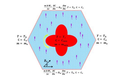
A novel treatment of fractional-time derivative using the incompressible smoothed particle hydrodynamics (ISPH) method is introduced to simulate the bioconvection flow of nano-enhanced phase change materials (NEPCM) in a porous hexagonal cavity. The fractional-time derivative is based on the Caputo style, which reflects the fractional order behavior in complex systems. In this work, the circular rotation of the embedded four-pointed star and the motion of oxytactic microorganisms in a hexagonal cavity are conducted. Due to the significance of fractional derivatives in handling real physical problems with more flexibility than conventional derivatives, the present scheme of the ISPH method is developed to solve the fractional-time derivative of the bioconvection flow in a porous hexagonal cavity. This study implicates the variations of a fractional-time derivative, a parametric of an inner four-pointed star, and the pertinent physical parameters on the behavior of a bioconvection flow of a nanofluid in a hexagonal-cavity containing oxytactic microorganisms. The presence of microorganisms has a significant role in many biological, engineering, and medical phenomena. From the present numerical investigation, it is well mentioned that the computational time of the transient processes can be reduced by applying a fractional-time derivative. The variable sizes of an inner four-pointed star enhance the bioconvection flow in a hexagonal cavity.

| [1] | S. U. S. Choi, J. A. Eastman, Enhancing thermal conductivity of fluids with nanoparticles, ASME International Mechanical Engineering Congress & Exposition, San Francisco, 1995. |
| [2] | S. K. Das, S. U. Choi, W. Yu, T. Pradeep, Nanofluids: science and technology, New York: John Wiley & Sons, 2007. |
| [3] |
J. A. Eastman, U. S. Choi, S. Li, L. J. Thompson, S. Lee, Enhanced thermal conductivity through the development of nanofluids, MRS Online Proceedings Library, 457 (1996), 3–11. https://doi.org/10.1557/PROC-457-3 doi: 10.1557/PROC-457-3

|
| [4] |
J. Buongiorno, L. W. Hu, Innovative technologies: two-phase heat transfer in water-based nanofluids for nuclear applications final report, Nuclear Engineering Education Research (NEER) Program, 2009. https://doi.org/10.2172/958216 doi: 10.2172/958216
|
| [5] |
N. Putra, Yanuar, F. N. Iskandar, Application of nanofluids to a heat pipe liquid-block and the thermoelectric cooling of electronic equipment, Exp. Therm. Fluid Sci., 35 (2011), 1274–1281. https://doi.org/10.1016/j.expthermflusci.2011.04.015 doi: 10.1016/j.expthermflusci.2011.04.015
|
| [6] |
O. Mahian, A. Kianifar, S. A. Kalogirou, I. Pop, S. Wongwises, A review of the applications of nanofluids in solar energy, Int. J. Heat Mass Tran., 57 (2013), 582–594. https://doi.org/10.1016/j.ijheatmasstransfer.2012.10.037 doi: 10.1016/j.ijheatmasstransfer.2012.10.037
|
| [7] |
S. Rashidi, O. Mahian, E. M. Languri, Applications of nanofluids in condensing and evaporating systems, J. Therm. Anal. Calorim., 131 (2018), 2027–2039. https://doi.org/10.1007/s10973-017-6773-7 doi: 10.1007/s10973-017-6773-7
|
| [8] |
M. A. Nazari, M. H. Ahmadi, M. Sadeghzadeh, M. B. Shafii, M. Goodarzi, A review on application of nanofluid in various types of heat pipes, J. Cent. South Univ., 26 (2019), 1021–1041. https://doi.org/10.1007/s11771-019-4068-9 doi: 10.1007/s11771-019-4068-9
|
| [9] |
J. Li, X. Zhang, B. Xu, M. Yuan, Nanofluid research and applications: a review, Int. J. Heat Mass Tran., 127 (2021), 105543. https://doi.org/10.1016/j.icheatmasstransfer doi: 10.1016/j.icheatmasstransfer
|
| [10] |
M. A. Sheremet, Applications of Nanofluids, Nanomaterials (Basel), 11 (2021), 1716. https://doi.org/10.3390/nano11071716 doi: 10.3390/nano11071716
|
| [11] |
A. V. Kuznetsov, The onset of thermo-bioconvection in a shallow fluid saturated porous layer heated from below in a suspension of oxytactic microorganisms, Eur. J. Mech. B-Fluid., 25 (2006), 223–233. https://doi.org/10.1016/j.euromechflu.2005.06.003 doi: 10.1016/j.euromechflu.2005.06.003
|
| [12] |
A. V. Kuznetsov, Nanofluid bioconvection in water-based suspensions containing nanoparticles and oxytactic microorganisms: oscillatory instability, Nanoscale Res. Lett., 6 (2011), 100. https://doi.org/10.1186/1556-276X-6-100 doi: 10.1186/1556-276X-6-100
|
| [13] |
A. J. Hillesdon, T. J. Pedley, Bioconvection in suspensions of oxytactic bacteria: linear theory, J. Fluid Mech., 324 (1996), 223–259. https://doi.org/10.1017/S0022112096007902 doi: 10.1017/S0022112096007902
|
| [14] |
T. J. Pedley, N. A. Hill, J. O. Kessler, The growth of bioconvection patterns in a uniform suspension of gyrotactic micro-organisms, J. Fluid Mech., 195 (1988), 223–237. https://doi.org/10.1017/S0022112088002393 doi: 10.1017/S0022112088002393
|
| [15] |
T. Yamamoto, Numerical simulation of the flows of phototactic microalgae suspensions in an illuminated circular channel, Nihon Reoroji Gakk., 43 (2015) 53–62. https://doi.org/10.1678/rheology.43.53 doi: 10.1678/rheology.43.53
|
| [16] |
M. A. Sheremet, I. Pop, Thermo-bioconvection in a square porous cavity filled by oxytactic microorganisms, Transp. Porous Med., 103 (2014), 191–205. https://doi.org/10.1007/s11242-014-0297-4 doi: 10.1007/s11242-014-0297-4
|
| [17] |
C. S. Balla, A. Ramesh, N. Kishan, A. M. Rashad, Z. M. A. Abdelrahman, Bioconvection in oxytactic microorganism-saturated porous square enclosure with thermal radiation impact, J. Therm. Anal. Calorim., 140 (2020), 2387–2395. https://doi.org/10.1007/s10973-019-09009-7 doi: 10.1007/s10973-019-09009-7
|
| [18] |
S. Ahmad, M. Ashraf, K. Ali, Bioconvection due to gyrotactic microbes in a nanofluid flow through a porous medium, Heliyon, 6 (2020), e05832. https://doi.org/10.1016/j.heliyon.2020.e05832 doi: 10.1016/j.heliyon.2020.e05832
|
| [19] |
D. K. Mandal, N. Biswas, N. K. Manna, R. S. R. Gorla, A. J. Chamkha, Role of surface undulation during mixed bioconvective nanofluid flow in porous media in presence of oxytactic bacteria and magnetic fields, Int. J. Mech. Sci., 211 (2021), 106778. https://doi.org/10.1016/j.ijmecsci.2021.106778 doi: 10.1016/j.ijmecsci.2021.106778
|
| [20] |
N. Biswas, D. K. Mandal, N. K. Manna, A. C. Benim, Magneto-hydrothermal triple-convection in a W-shaped porous cavity containing oxytactic bacteria, Sci. Rep., 12 (2022), 18053. https://doi.org/10.1038/s41598-022-18401-7 doi: 10.1038/s41598-022-18401-7
|
| [21] |
M. Habibishandiz, Z. Saghir, MHD mixed convection heat transfer of nanofluid containing oxytactic microorganisms inside a vertical annular porous cylinder, International Journal of Thermofluids, 14 (2022), 100151. https://doi.org/10.1016/j.ijft.2022.100151 doi: 10.1016/j.ijft.2022.100151
|
| [22] |
S. Hussain, A. M. Aly, H. F. Öztop, Magneto-bioconvection flow of hybrid nanofluid in the presence of oxytactic bacteria in a lid-driven cavity with a streamlined obstacle, Int. Commun. Heat Mass, 134 (2022), 106029. https://doi.org/10.1016/j.icheatmasstransfer.2022.106029 doi: 10.1016/j.icheatmasstransfer.2022.106029
|
| [23] |
A. M. Rashad, H. A. Nabwey, Gyrotactic mixed bioconvection flow of a nanofluid past a circular cylinder with convective boundary condition, J. Taiwan Inst. Chem. E., 99 (2019), 9–17. https://doi.org/10.1016/j.jtice.2019.02.035 doi: 10.1016/j.jtice.2019.02.035
|
| [24] |
B. P. Geridonmez, H. F. Oztop, Conjugate natural convection flow of a nanofluid with oxytactic bacteria under the effect of a periodic magnetic field, J. Magn. Magn. Mater., 564 (2022), 170135. https://doi.org/10.1016/j.jmmm.2022.170135 doi: 10.1016/j.jmmm.2022.170135
|
| [25] |
B. Chen, X. Wang, R. Zeng, Y. Zhang, X. Wang, J. Niu, et al., An experimental study of convective heat transfer with microencapsulated phase change material suspension: Laminar flow in a circular tube under constant heat flux, Exp. Therm. Fluid Sci., 32 (2008), 1638–1646. https://doi.org/10.1016/j.expthermflusci.2008.05.008 doi: 10.1016/j.expthermflusci.2008.05.008
|
| [26] |
W. Wu, H. Bostanci, L. C. Chow, Y. Hong, C. M. Wang, M. Su, et al., Heat transfer enhancement of PAO in microchannel heat exchanger using nano-encapsulated phase change indium particles, Int. J. Heat Mass Tran., 58 (2013), 348–355. https://doi.org/10.1016/j.ijheatmasstransfer.2012.11.032 doi: 10.1016/j.ijheatmasstransfer.2012.11.032
|
| [27] |
C. J. Smith, P. M. Forster, R. Crook, Global analysis of photovoltaic energy output enhanced by phase change material cooling, Appl. Energ., 126 (2014), 21–28. https://doi.org/10.1016/j.apenergy.2014.03.083 doi: 10.1016/j.apenergy.2014.03.083
|
| [28] |
W. Su, J. Darkwa, G. Kokogiannakis, Review of solid-liquid phase change materials and their encapsulation technologies, Renew. Sust. Energ. Rev., 48 (2015), 373–391. https://doi.org/10.1016/j.rser.2015.04.044 doi: 10.1016/j.rser.2015.04.044
|
| [29] |
Y. Pahamli, M. J. Hosseini, A. A. Ranjbar, R. Bahrampoury, Analysis of the effect of eccentricity and operational parameters in PCM-filled single-pass shell and tube heat exchangers, Renew. Energ., 97 (2016), 344–357. https://doi.org/10.1016/j.renene.2016.05.090 doi: 10.1016/j.renene.2016.05.090
|
| [30] |
C. Liu, Z. Rao, J. Zhao, Y. Huo, Y. Li, Review on nanoencapsulated phase change materials: Preparation, characterization and heat transfer enhancement, Nano Energy, 13 (2015), 814–826. https://doi.org/10.1016/j.nanoen.2015.02.016 doi: 10.1016/j.nanoen.2015.02.016
|
| [31] |
H. R. Seyf, Z. Zhou, H. B. Ma, Y. Zhang, Three dimensional numerical study of heat-transfer enhancement by nano-encapsulated phase change material slurry in microtube heat sinks with tangential impingement, Int. J. Heat Mass Tran., 56 (2013), 561–573. https://doi.org/10.1016/j.ijheatmasstransfer.2012.08.052 doi: 10.1016/j.ijheatmasstransfer.2012.08.052
|
| [32] |
M. Ghalambaz, S. A. M. Mehryan, I. Zahmatkesh, A. Chamkha, Free convection heat transfer analysis of a suspension of nano-encapsulated phase change materials (NEPCMs) in an inclined porous cavity, Int. J. Therm. Sci., 157 (2020), 106503. https://doi.org/10.1016/j.ijthermalsci.2020.106503 doi: 10.1016/j.ijthermalsci.2020.106503
|
| [33] |
S. A. M. Mehryan, M. Ismael, M. Ghalambaz, Local thermal nonequilibrium conjugate natural convection of nano-encapsulated phase change particles in a partially porous enclosure, Math. Method. Appl. Sci., 2020 (2020), 6338. https://doi.org/10.1002/mma.6338 doi: 10.1002/mma.6338
|
| [34] |
S. Hussain, N. Alsedias, A. M. Aly, Natural convection of a water-based suspension containing nano-encapsulated phase change material in a porous grooved cavity, J. Energy Storage, 51 (2022), 104589. https://doi.org/10.1016/j.est.2022.104589 doi: 10.1016/j.est.2022.104589
|
| [35] |
C. J. Ho, Y. C. Liu, T. F. Yang, M. Ghalambaz, W. M. Yan, Convective heat transfer of nano-encapsulated phase change material suspension in a divergent minichannel heatsink, Int. J. Heat Mass Tran., 165 (2021), 120717. https://doi.org/10.1016/j.ijheatmasstransfer.2020.120717 doi: 10.1016/j.ijheatmasstransfer.2020.120717
|
| [36] |
R. A. Gingold, J. J. Monaghan, Smoothed particle hydrodynamics: theory and application to non-spherical stars, Mon. Not. R. Astron. Soc., 181 (1977), 375–389. https://doi.org/10.1093/mnras/181.3.375 doi: 10.1093/mnras/181.3.375
|
| [37] |
L. B. Lucy, A numerical approach to the testing of the fission hypothesis, Astron. J., 82 (1977), 1013–1024. https://doi.org/10.1086/112164 doi: 10.1086/112164
|
| [38] |
S. J. Cummins, M. Rudman, An SPH projection method, J. Comput. Phys., 152 (1999), 584–607. https://doi.org/10.1006/jcph.1999.6246 doi: 10.1006/jcph.1999.6246
|
| [39] |
M. Asai, A. M. Aly, Y. Sonoda, Y. Sakai, A stabilized incompressible SPH method by relaxing the density invariance condition, J. Appl. Math., 2012 (2012), 139583. https://doi.org/10.1155/2012/139583 doi: 10.1155/2012/139583
|
| [40] |
F. Garoosi, A. Shakibaeinia, Numerical simulation of entropy generation due to natural convection heat transfer using Kernel Derivative-Free (KDF) Incompressible Smoothed Particle Hydrodynamics (ISPH) model, Int. J. Heat Mass Tran., 150 (2020), 119377. https://doi.org/10.1016/j.ijheatmasstransfer.2020.119377 doi: 10.1016/j.ijheatmasstransfer.2020.119377
|
| [41] |
A. M. Aly, Mixing between solid and fluid particles during natural convection flow of a nanofluid-filled H-shaped cavity with three center gates using ISPH method, Int. J. Heat Mass Tran., 157 (2020), 119803. https://doi.org/10.1016/j.ijheatmasstransfer.2020.119803 doi: 10.1016/j.ijheatmasstransfer.2020.119803
|
| [42] |
A. M. Aly, A. M. Yousef, N. Alsedais, MHD double diffusion of a nanofluid within a porous annulus using a time fractional derivative of the ISPH method, Int. J. Mod. Phys. C, 33 (2021), 2250056. https://doi.org/10.1142/S0129183122500565 doi: 10.1142/S0129183122500565
|
| [43] |
Y. Shimizu, H. Gotoh, A. Khayyer, K. Kita, Fundamental investigation on the applicability of higher-order consistent ISPH method, Int. J. Offshore Polar, 32 (22022), 275–284. https://doi.org/10.17736/ijope.2022.jc868 doi: 10.17736/ijope.2022.jc868
|
| [44] |
A. M. Salehizadeh, A. R. Shafiei, A coupled ISPH-TLSPH method for simulating fluid-elastic structure interaction problems, J. Marine. Sci. Appl., 21 (2022), 15–36. https://doi.org/10.1007/s11804-022-00260-3 doi: 10.1007/s11804-022-00260-3
|
| [45] |
N. Alsedais, A. Al-Hanaya, A. M. Aly, Magneto-bioconvection flow in a porous annulus between circular cylinders containing oxytactic microorganisms and NEPCM, Int. J. Numer. Method. H., 33 (2023), 3228–3254. https://doi.org/10.1108/HFF-02-2023-0095 doi: 10.1108/HFF-02-2023-0095
|
| [46] |
W. Alhejaili, A. M. Aly, Magneto-bioconvection flow in an annulus between circular cylinders containing oxytactic microorganisms, Int. Commun. Heat Mass, 146 (2023), 106893. https://doi.org/10.1016/j.icheatmasstransfer.2023.106893 doi: 10.1016/j.icheatmasstransfer.2023.106893
|
| [47] |
A. Alaria, A. M. Khan, D. L. Suthar, D. Kumar, Application of fractional operators in modelling for charge carrier transport in amorphous semiconductor with multiple trapping, Int. J. Appl. Comput. Math., 5 (2019), 167. https://doi.org/10.1007/s40819-019-0750-8 doi: 10.1007/s40819-019-0750-8
|
| [48] |
M. M. A. Khater, D. Baleanu, On abundant new solutions of two fractional complex models, Adv. Differ. Equ., 2020 (2020), 268. https://doi.org/10.1186/s13662-020-02705-x doi: 10.1186/s13662-020-02705-x
|
| [49] |
A. Hyder, A. H. Soliman, A new generalized θ-conformable calculus and its applications in mathematical physics, Phys. Scr., 96 (2020), 015208. https://doi.org/10.1088/1402-4896/abc6d9 doi: 10.1088/1402-4896/abc6d9
|
| [50] |
A. Hyder, M. A. Barakat, Novel improved fractional operators and their scientific applications, Adv. Differ. Equ., 2021 (2021), 389. https://doi.org/10.1186/s13662-021-03547-x doi: 10.1186/s13662-021-03547-x
|
| [51] |
A. Hyder, M. A. Barakat, A. Fathallah, C. Cesarano, Further integral inequalities through some generalized fractional integral operators, Fractal Fract., 5 (2021), 282. https://doi.org/10.3390/fractalfract5040282 doi: 10.3390/fractalfract5040282
|
| [52] |
T. Abdeljawad, On conformable fractional calculus, J. Comput. Appl. Math., 279 (2015), 57–66. https://doi.org/10.1016/j.cam.2014.10.016 doi: 10.1016/j.cam.2014.10.016
|
| [53] |
M. Ghalambaz, A. J. Chamkha, D. Wen, Natural convective flow and heat transfer of Nano-Encapsulated Phase Change Materials (NEPCMs) in a cavity, Int. J. Heat Mass Tran., 138 (2019), 738–749. https://doi.org/10.1016/j.ijheatmasstransfer.2019.04.037 doi: 10.1016/j.ijheatmasstransfer.2019.04.037
|
| [54] | I. Podlubny, Fractional differential equations: An introduction to fractional derivatives, fractional differential equations, to methods of their solution and some of their applications, San Diego: Academic Press, 1999. |
| [55] |
Ş. Toprakseven, Numerical solutions of conformable fractional differential equations by Taylor and finite difference methods, Süleyman Demirel Üniversitesi Fen Bilimleri Enstitüsü Dergisi, 23 (2019), 850–863. https://doi.org/10.19113/sdufenbed.579361 doi: 10.19113/sdufenbed.579361
|


Figures(15) / Tables(1)

Abdelraheem M. Aly, Abd-Allah Hyder. Fractional-time derivative in ISPH method to simulate bioconvection flow of a rotated star in a hexagonal porous cavity[J]. AIMS Mathematics, 2023, 8(12): 31050-31069. doi: 10.3934/math.20231589


 DownLoad: