Derivation of an approximate formula of the Rabotnov fractional-exponential kernel fractional derivative and applied for numerically solving the blood ethanol concentration system

Ahmed F. S. Aboubakr; Gamal M. Ismail; Mohamed M. Khader; Mahmoud A. E. Abdelrahman; Ahmed M. T. AbdEl-Bar; Mohamed Adel; Ahmed F. S. Aboubakr; Gamal M. Ismail; Mohamed M. Khader; Mahmoud A. E. Abdelrahman; Ahmed M. T. AbdEl-Bar; Mohamed Adel

doi:10.3934/math.20231569

AIMS Mathematics

2023, Volume 8, Issue 12: 30704-30716. doi: 10.3934/math.20231569

Previous Article Next Article

Research article Special Issues

Derivation of an approximate formula of the Rabotnov fractional-exponential kernel fractional derivative and applied for numerically solving the blood ethanol concentration system

1.
Department of Mathematics, College of Science, Taibah University, Medina 41411, Saudi Arabia
2.
Department of Mathematics, University of Fayoum, Fayoum 63514, Egypt
3.
Department of Mathematics, Faculty of Science, Islamic University of Madinah, Medina 42210, Saudi Arabia
4.
Department of Mathematics and Statistics, College of Science, Imam Mohammad Ibn Saud Islamic University (IMSIU), Riyadh 11566, Saudi Arabia
5.
Department of Mathematics, Faculty of Science, Benha University, Benha 13518, Egypt
6.
Department of Mathematics, Faculty of Science, Mansoura University, Mansoura 35516, Egypt
7.
Department of Mathematics, Faculty of Science, Tanta University, Tanta 31527, Egypt
8.
Department of Mathematics, Faculty of Science, Cairo University, Giza 12613, Egypt

Received: 11 September 2023 Revised: 31 October 2023 Accepted: 02 November 2023 Published: 14 November 2023
MSC : 41A10, 65N12, 65N35

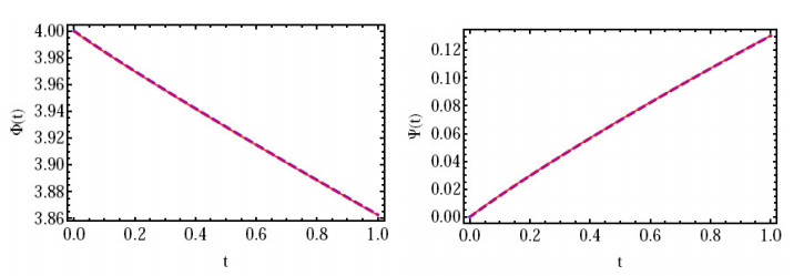
The article aimed to develop an accurate approximation of the fractional derivative with a non-singular kernel (the Rabotnov fractional-exponential formula), and show how to use it to solve numerically the blood ethanol concentration system. This model can be represented by a system of fractional differential equations. First, we created a formula for the fractional derivative of a polynomial function $t^{p}$ using the Rabotnov exponential kernel. We used the shifted Vieta-Lucas polynomials as basis functions on the spectral collocation method in this work. By solving the specified model, this technique generates a system of algebraic equations. We evaluated the absolute and relative errors to estimate the accuracy and efficiency of the given procedure. The results point to the technique's potential as a tool for numerically treating these models.

Keywords:

Citation: Ahmed F. S. Aboubakr, Gamal M. Ismail, Mohamed M. Khader, Mahmoud A. E. Abdelrahman, Ahmed M. T. AbdEl-Bar, Mohamed Adel. Derivation of an approximate formula of the Rabotnov fractional-exponential kernel fractional derivative and applied for numerically solving the blood ethanol concentration system[J]. AIMS Mathematics, 2023, 8(12): 30704-30716. doi: 10.3934/math.20231569

Related Papers:

[1]	Ahmed E. Abouelregal, Faisal Alsharif, Hashem Althagafi, Yazeed Alhassan . Fractional heat transfer DPL model incorporating an exponential Rabotnov kernel to study an infinite solid with a spherical cavity. AIMS Mathematics, 2024, 9(7): 18374-18402. doi: 10.3934/math.2024896
[2]	Jagdev Singh, Jitendra Kumar, Devendra kumar, Dumitru Baleanu . A reliable numerical algorithm based on an operational matrix method for treatment of a fractional order computer virus model. AIMS Mathematics, 2024, 9(2): 3195-3210. doi: 10.3934/math.2024155
[3]	Jagdev Singh, Jitendra Kumar, Devendra Kumar, Dumitru Baleanu . A reliable numerical algorithm for fractional Lienard equation arising in oscillating circuits. AIMS Mathematics, 2024, 9(7): 19557-19568. doi: 10.3934/math.2024954
[4]	Younes Talaei, Sanda Micula, Hasan Hosseinzadeh, Samad Noeiaghdam . A novel algorithm to solve nonlinear fractional quadratic integral equations. AIMS Mathematics, 2022, 7(7): 13237-13257. doi: 10.3934/math.2022730
[5]	Zunyuan Hu, Can Li, Shimin Guo . Fast finite difference/Legendre spectral collocation approximations for a tempered time-fractional diffusion equation. AIMS Mathematics, 2024, 9(12): 34647-34673. doi: 10.3934/math.20241650
[6]	Waleed Mohamed Abd-Elhameed, Abdullah F. Abu Sunayh, Mohammed H. Alharbi, Ahmed Gamal Atta . Spectral tau technique via Lucas polynomials for the time-fractional diffusion equation. AIMS Mathematics, 2024, 9(12): 34567-34587. doi: 10.3934/math.20241646
[7]	Manal Alqhtani, Khaled M. Saad . Numerical solutions of space-fractional diffusion equations via the exponential decay kernel. AIMS Mathematics, 2022, 7(4): 6535-6549. doi: 10.3934/math.2022364
[8]	M. Adel, M. M. Khader, Hijaz Ahmad, T. A. Assiri . Approximate analytical solutions for the blood ethanol concentration system and predator-prey equations by using variational iteration method. AIMS Mathematics, 2023, 8(8): 19083-19096. doi: 10.3934/math.2023974
[9]	Imran Talib, Md. Nur Alam, Dumitru Baleanu, Danish Zaidi, Ammarah Marriyam . A new integral operational matrix with applications to multi-order fractional differential equations. AIMS Mathematics, 2021, 6(8): 8742-8771. doi: 10.3934/math.2021508
[10]	M. A. Zaky, M. Babatin, M. Hammad, A. Akgül, A. S. Hendy . Efficient spectral collocation method for nonlinear systems of fractional pantograph delay differential equations. AIMS Mathematics, 2024, 9(6): 15246-15262. doi: 10.3934/math.2024740

Abstract

1. Introduction

Numerous authors have remained interested in fractional calculus throughout the past three decades ^[1]. To addresFresea s the demand for models of real-world problems in numerous domains, researchers have identified the importance of discrete fractional derivatives with unique, singular, or non-singular, distinct kernels ^[2,3]. Due to the lack of an exact solution in the majority of fractional differential equations (FDEs), numerical and approximation techniques must be used ^[4,5,6,7]. Also, for more details, you can read ^[8,9,10].

As generalizations of the classical ones, a wide range of fractional operators have been developed recently. The typical derivative's power kernel, as shown by Caputo and Riemann-Liouville, a novel class of fractional derivatives is produced when the exponential and Mittag-Leffler kernels are used to replace this kernel. Atangana-Baleanu, and Caputo-Fabrizio, respectively, are the names of the derivatives with Mittag-Leffler and exponential kernels. Numerous fields, such as chaos theory ^[11], medical sciences ^{[12,13,14,15,16]} and groundwater flow ^[17], make extensive use of these non-singular derivatives ^[18].

It is difficult to create a higher-order convergent method to solve numerically the multidimensional FDEs. Due to such reasons, some numerical methods are frequently applied to achieve this objective. Among them, is the space-time spectral order sinc-collocation method, which is used for solving the fourth-order nonlocal heat model arising in viscoelasticity ^[19]. Also, the numerical solution of the three-dimensional nonlocal evolution equation with a weakly singular kernel is considered where the first-order fractional convolution quadrature scheme and backward Euler alternating direction implicit (ADI) method, are proposed to approximate and discretize the Riemann-Liouville fractional integral term and temporal derivative, respectively. To obtain a fully discrete method, the standard central finite difference scheme is used to discretize the second-order spatial derivative. By using the ADI scheme for the three-dimensional problem, the overall computational cost is reduced significantly ^[20].

Here in this paper, a broad approximation analytical method for locating the approximate solution of the differential equations is the spectral collocation technique (SCM). The well-known polynomials on [-2, 2], known as Vieta-Lucas polynomials, have various applications. They are commonly utilized because they have high function approximation qualities. SCM provides certain benefits for dealing with FDEs because any of the numerical programs can readily produce the Vieta-Lucas coefficients for the solution. This makes the procedure quicker than the alternatives. Additionally, this approach is a numerical strategy for solving many problems in both finite and infinite domains ^[21,22,23].

This effort will estimate the fractional operator using the Rabotnov fractional-exponential (RFE) kernel. The fractional order derivative of a polynomial function $t^{p}$ is first estimated using the RFE kernel. Based on this approximation and the properties of the Vieta-Lucas polynomials (VLPs), we offer a numerical simulation for the suggested model. By using the polynomial's fractional derivative, we can demonstrate the accuracy of this new formula. We also investigate the blood ethanol concentration system (BECS) with the RFE kernel fractional derivative, allowing us to confidently forecast the outcome of our approach.

The rest of the paper is organized as follows: In Section 2, we present some definitions and concepts concerning fractional derivatives, the approximation of fractional order derivative of $t^{p}$ , and the shifted Vieta-Lucas polynomials. Through Section 3, we give the implementation of the proposed method. In Section 4, we present a numerical simulation of the proposed model under study. Finally, the conclusions are in Section 5.

2. Definitions and concepts

2.1. Fractional derivatives

Definition 2.1. Let $\varphi(t)\in H^{1}(0, b)$ , then the fractional Caputo derivative $^{C}D^{\nu}$ of order $0 < \nu\leq1$ is given by

$^{C}D^{\nu}\varphi(t) = \frac{1}{\Gamma(1-\nu)}\, \int_{0}^{t}\frac{\varphi^{'}(\tau)}{(t-\tau)^{\nu}}d\tau,\quad t > 0.$

Definition 2.2. The Caputo fractional derivative (left-sided) on interval $[0, 1]$ for a function $\Theta(t)$ of order $\beta$ is defined by

$\begin{equation} ^{RFE}D^{\beta}\Theta(t) = \int_{0}^{t}\,\Theta^{(n)}(\xi)\,\mathbb{Re}_{\beta}[-\Omega(t-\xi)^{\beta}]d\xi,\quad n-1 < \beta\leq n, \end{equation}$

(2.1)

where $\Omega\in\, R^{+}$ and the Rabotnov fractional exponential function is defined by

$\mathbb{Re}_{\beta}[-\Omega(t)^{\beta}] = \sum\limits_{k = 0}^{\infty}\frac{(-\Omega)^{k}\,t^{(k+1)(\beta+1)-1}}{\Gamma[(k+1)(\beta+1)]}.$

Regarding the RFE-operator derivative, further information can be found in ^[24,25].

2.2. Approximation of fractional order derivative of $t^{p}$

In this part, an approximate fractional derivative formula corresponding to the RFE kernel is computed using a widely accessible numerical integration scheme, such as the Simpson- $\frac{1}{3}$ rule.

Theorem 2.1. ^[26] For $n-1 < \beta < n$ and $g(t) = t^{p}$ with $p\geq n$ ( $n = \lceil\beta\rceil$ ), we have

$\begin{equation} \begin{split} ^{RFE}D^{\beta}\,t^{p} = \frac{h\Gamma(p+1)}{3\Gamma(p+1-\lceil\beta\rceil)}\Big{[}G_{\beta,p}(t,\xi_{0})+G_{\beta,p}(t,\xi_{N}) +4\,\sum\limits_{k = 1,\,k-odd}^{N-1}\,G_{\beta,p}(t,\xi_{k})+2\,\sum\limits_{k = 2,\,k-even}^{N-2}\,G_{\beta,p}(t,\xi_{k})\Big{]}, \end{split} \end{equation}$

(2.2)

where the domain $[0, 1]$ is divided into $N$ equal segments and the length of each segment is $h$ :

$h = \frac{1}{N},\quad G_{\beta,p}(t,\xi) = \xi^{p-\lceil\beta\rceil}\,\mathbb{Re}_{\beta}[-\Omega(t-\xi)^{\beta}],\quad \xi_{k} = \frac{k}{N},\quad k = 0,1,2,...,N.$

Remark 2.1. Due to the difficulty of integration (2.1), it was evaluated using Simpson's 1/3 rule, or any other numerical method could be used. We did not use the trapezoidal rule, due to the hope of getting the numerical solutions with small errors, which will not be achieved unless a highly accurate method of integration is used. Here in our work we will express the solution as a finite series of polynomials, and as it shows, we can get more accurate values if we increase the order of approximation. This, in turn, prompts us to use high-precision integration techniques, such as the Simpson rule or others.

2.3. The shifted VLPs

To achieve our goal, we present in this subsection the fundamental definitions, notations and characteristics of the shifted VLPs ^[27]. The majority of our research is concentrated on an orthogonal polynomials class. The recurrence relations and analytical forms of these polynomials can be used to construct a new family of orthogonal polynomials called VLPs.

VLPs $\mathrm{VL}_{k}(z)$ of degree $k \in \mathbb{N}_{0}$ is defined as follows ^[27]:

$\mathrm{VL}_{k}(z) = 2 \cos (k \psi), \quad \psi = \arccos(0.5z),\quad \psi\in[0, \pi], \quad |z| \leq 2.$

The $\mathrm{VL}_{k}(z)$ satisfies

$\mathrm{VL}_{k}(z) = z \mathrm{VL}_{k-1}(z)-\mathrm{VL}_{k-2}(z), \quad k = 2,3, \ldots, \quad \mathrm{VL}_{0}(z) = 2, \quad \mathrm{VL}_{1}(z) = z.$

Using $z = 4t-2$ , VLPs are used to create a new class of orthogonal polynomials on $[0, 1]$ , which will be designated by $\mathrm{VL}_{k}^{s}(t)$ and so

$\mathrm{VL}_{k}^{s}(t) = \mathrm{VL}_{k}(4 t-2).$

$\mathrm{VL}_{k}^{s}(t)$ has the following recurrence relation:

$\mathrm{VL}_{k+1}^{s}(t) = (4 t-2) \mathrm{VL}_{k-1}^{s}(t)-\mathrm{VL}_{k-2}^{s}(t), \quad k = 2,3, \ldots,$

where $\mathrm{VL}_{0}^{s}(t) = 2, \, \, \mathrm{VL}_{1}^{s}(t) = 4 t-2.$ Also, we find $\mathrm{VL}_{k}^{s}(0) = 2(-1)^{k}$ and $\mathrm{VL}_{k}^{s}(1) = 2, \, \, k = 0, 1, 2, ...\, .$ The analytical formula for $\mathrm{VL}_{k}^{s}(t)$ is

$\mathrm{VL}_{k}^{s}(t) = 2 k \sum\limits_{j = 0}^{k}(-1)^{j} \frac{4^{k-j} \Gamma(2 k-j)}{\Gamma(j+1) \Gamma(2 k-2 j+1)} \,t^{k-j}, \quad k = 2,3, \ldots\; .$

The polynomials $\mathrm{VL}_{i}^{s}(t)$ are orthogonal on $[0, 1]$ w.r.t. the weight function $\frac{1}{\sqrt{t-t^{2}}}$ , and so we have

$\langle\mathrm{VL}_{i}^{s}(t), \mathrm{VL}_{j}^{s}(t)\rangle = \int_{0}^{1} \frac{\mathrm{VL}_{i}^{s}(t) \mathrm{VL}_{j}^{s}(t)}{\sqrt{t-t^{2}}} d t = \left\{\begin{array}{ll} 0, & i \neq j \neq 0, \\ 4 \pi, & i = j = 0, \\ 2 \pi, & i = j \neq 0. \end{array}\right.$

Let $v(t) \in L^2 [0, 1]$ , then,

$\begin{equation} v(t) = \sum\limits_{j = 0}^{\infty} c_{j} \mathrm{VL}_{j}^{s}(t). \end{equation}$

(2.3)

Using the first $m+1$ terms of (2.3), we have

$\begin{equation} v_{m}(t) = \sum\limits_{j = 0}^{m} c_{j} \mathrm{VL}_{j}^{s}(t), \end{equation}$

(2.4)

where $c_{j}, j = 0, 1, 2, \ldots, m$ can be obtained by

$\begin{equation} c_{j} = \frac{1}{\delta_{j}} \int_{0}^{1} \frac{v_{m}(t) \mathrm{VL}_{j}^{s}(t)}{\sqrt{t-t^{2}}}\,dt,\quad\quad\quad \delta_{j} = \left\{\begin{array}{ll} 4 \pi, &\quad j = 0, \\ 2 \pi, &\quad j = 1,2, \ldots, m. \end{array}\right. \end{equation}$

(2.5)

Lemma 2.1. If $v(t)\in\, L_{\tilde{\textbf{w}}}^{2}\, [0, 1]$ w.r.t. the weight function $\tilde{\textbf{w}}(t) = \frac{1}{\sqrt{t-t^2}}$ , and $|v''(t)|\leq\varepsilon, \, \, \varepsilon \in \mathbb{R}$ , then the approximation (2.4) converges uniformly to $v(t)$ as $m \rightarrow \infty$ . Furthermore, we have the following estimations:

(1)

$\left|c_{j}\right| \leq \frac{\varepsilon}{4 j\left(j^{2}-1\right)}, \quad j > 2.$

(2) The error can be estimated by

$\left\|v(t)-v_{m}(t)\right\|_{\tilde{\textbf{w}}} < \frac{L}{12\,\sqrt{m^{3}}}.$

(3) If $v^{(m)}(t)\in\, C[0, 1]$ , then,

$\left\|v(t)-v_{m}(t)\right\| \leq \frac{\Delta\, \Pi^{m+1}}{(m+1) !} \sqrt{\pi},\quad \Delta = \max _{t \in[0,1]}\,v^{(m+1)}(t) \,\,\,\hbox{and} \,\,\, \Pi = \max \left\{1-t_{0}, t_{0}\right\}.$

Proof. The details of the proof for these three items in this lemma can be found through Theorems 2–4 in ^[28]. □

For additional information on the convergence analysis of the approximation (2.4), and the VLPs see ^[29].

Theorem 2.2. The $\beta$ -order of the RFE fractional derivative for $v_{i}(t)$ which is given in Eq (2.4) can be found by ^[26]:

$\begin{equation} \begin{split} ^{RFE}D^{\beta}\,v_{i}(t) = \sum\limits_{j = \lceil\beta\rceil}^{i}\,\chi_{i, j,\beta}\Big{[}G_{\beta,p}(t,\xi_{0})+G_{\beta,p}(t,\xi_{m}) +4\,\sum\limits_{k = 1,\,k-odd}^{m-1}\,G_{\beta,p}(t,\xi_{k})+2\,\sum\limits_{k = 2,\,k-even}^{m-2}\,G_{\beta,p}(t,\xi_{k})\Big{]}, \end{split} \end{equation}$

(2.6)

where

$\chi_{i, j,\beta} = \frac{h\,\Gamma(i-j+1)}{3\,\Gamma(i-j+1-\lceil\beta\rceil)}\times\frac{(-1)^{j} 2i\,4^{i-j} \Gamma(2 i-j)}{\Gamma(j+1) \Gamma(2 i-2 j+1)},\quad G_{\beta,p}(t,\xi) = \xi^{p-\lceil\beta\rceil}\,\mathbb{Re}_{\beta}[-\Omega(t-\xi)^{\beta}]_{p = i-j}.$

Proof. Since the fractional operator $^{RFE}D^{\beta}$ is linear, so from (2.4), we can obtain the following:

$\begin{equation} \begin{split} ^{RFE}D^{\beta}\,v_{i}(t)& = \sum\limits_{j = 0}^{i}\frac{(-1)^{j} 2i\,4^{i-j} \Gamma(2 i-j)}{\Gamma(j+1) \Gamma(2 i-2 j+1)}\,^{RFE}D^{\beta}\,t^{i-j}. \end{split} \end{equation}$

(2.7)

Now, from Theorem 2.1, we can get the following:

$\begin{equation} \begin{split} ^{RFE}D^{\beta}\,t^{i-j} = &\frac{\Gamma(i-j+1)}{\Gamma(i-j-\lceil\beta\rceil+1)}\times\frac{h}{3}\Big{[}G_{\beta,p}(t,\xi_{0})+G_{\beta,p}(t,\xi_{N})\\& +4\,\sum\limits_{k = 1,\,k-odd}^{N-1}\,G_{\beta,p}(t,\xi_{k})+2\,\sum\limits_{k = 2,\,k-even}^{N-2}\,G_{\beta,p}(t,\xi_{k})\Big{]}, \end{split} \end{equation}$

(2.8)

where the domain $[0, 1]$ is divided into $m$ equal segments with length $h$ of each segment:

$h = \frac{1}{N},\quad G_{\beta,p}(t,\xi) = \xi^{p-\lceil\beta\rceil}\,\mathbb{Re}_{\beta}[-\Omega(t-\xi)^{\beta}]_{p = i-j},\quad \xi_{k} = \frac{k}{N},\quad k = 0,1,2,...,N.$

Connecting (2.7) and (2.8), we get

$\begin{equation} \begin{split} ^{RFE}D^{\beta}\,v_{i}(t)& = \sum\limits_{j = \lceil\beta\rceil}^{i}\frac{\Gamma(i-j+1)}{\Gamma(i-j+1-\lceil\beta\rceil)}\times\frac{(-1)^{j} 2i\,4^{i-j} \Gamma(2 i-j)}{\Gamma(j+1) \Gamma(2 i-2 j+1)}\times\frac{h}{3}\Big{[}G_{\beta,p}(t,\xi_{0})+G_{\beta,p}(t,\xi_{N})\\& \quad +4\,\sum\limits_{k = 1,\,k-odd}^{N-1}\,G_{\beta,p}(t,\xi_{k})+2\,\sum\limits_{k = 2,\,k-even}^{N-2}\,G_{\beta,p}(t,\xi_{k})\Big{]}. \end{split} \end{equation}$

(2.9)

The proof is complete because of this finding, which makes it simple to arrive at the necessary formula (2.6). □

3. Implementation of the proposed method

This section focuses on determining the alcohol concentrations in a person's blood $\Psi(t)$ and stomach $\Phi(t)$ . The primary source of the actual data used in the current research study was an experimental investigation conducted in ^[30]. The proposed model is offered and based on the kinetic reaction of the RFE fractional derivative in the following form:

$\begin{equation} \,^{RFE}D^{\theta}\,\Phi(t) = -\lambda^{\theta} \Phi(t), \end{equation}$

(3.1)

$\begin{equation} ^{RFE}D^{\nu}\,\Psi(t) = \lambda^{\nu} \Phi(t)-\mu^{\nu} \Psi(t), \end{equation}$

(3.2)

$\begin{equation} \Phi(0) = \Phi_{0},\quad\quad\quad \Psi(0) = 0, \end{equation}$

(3.3)

where the parameters are defined in ^[30]. The exact solution of (3.1)–(3.3) is given by ^[31]:

$\begin{equation} \begin{split} &\Phi(t) = \Phi_{0}\,E_{\theta}(-\lambda^{\theta}t^{\theta}),\\& \Psi(t) = \Phi_{0}\,\lambda^{\nu}\sum\limits_{r = 0}^{\infty}\sum\limits_{q = 0}^{\infty} \frac{(-\lambda^{\theta})^{r}(-\mu^{\nu})^{q}}{\Gamma(r\,\theta+q\,\nu+\nu+1)}t^{r\,\theta+q\,\nu+\nu}. \end{split} \end{equation}$

(3.4)

Now, we use the SCM to numerically solve (3.1)–(3.3). $\Phi(t)$ and $\Psi(t)$ can be approximated by $\Phi_{m}(t)$ and $\Psi_{m}(t)$ , respectively as follows:

$\begin{equation} \Phi_{m}(t) = \sum\limits_{i = 0}^{m}\,\rho_{i}\,\mathrm{VL}_{i}^{s}(t),\quad\quad \Psi_{m}(t) = \sum\limits_{i = 0}^{m}\,\sigma_{i}\,\mathrm{VL}_{i}^{s}(t). \end{equation}$

(3.5)

Using (3.1), (3.2), (3.5) and (2.6), then,

$\begin{equation} \begin{split} &\sum\limits_{j = \lceil\theta\rceil}^{m}\,\rho_{j}\,\chi_{m, j,\theta}\Big{[}G_{\theta,p}(t,\xi_{0})+G_{\theta,p}(t,\xi_{N}) +4\,\sum\limits_{k = 1,\,k-odd}^{N-1}\,G_{\theta,p}(t,\xi_{k})+2\,\sum\limits_{k = 2,\,k-even}^{N-2}\,G_{\theta,p}(t,\xi_{k})\Big{]}\\ = &-\left(\lambda^{\theta}\sum\limits_{i = 0}^{m}\,\rho_{i}\,\mathrm{VL}_{i}^{s}(t)\right), \end{split} \end{equation}$

(3.6)

$\begin{equation} \begin{split} &\sum\limits_{j = \lceil\nu\rceil}^{m}\,\sigma_{j}\,\chi_{m, j,\nu}\Big{[}G_{\nu,p}(t,\xi_{0})+G_{\nu,p}(t,\xi_{N})+4\,\sum\limits_{k = 1,\,k-odd}^{N-1}\,G_{\nu,p}(t,\xi_{k})+2\,\sum\limits_{k = 2,\,k-even}^{N-2}\, G_{\nu,p}(t,\xi_{k})\Big{]}\\ = &\lambda^{\nu}\left(\sum\limits_{i = 0}^{m}\,\rho\,_{i}\,\mathrm{VL}_{i}^{s}(t)\right)-\mu^{\nu}\left(\sum\limits_{i = 0}^{m} \,\sigma_{i}\,\mathrm{VL}_{i}^{s}(t)\right). \end{split} \end{equation}$

(3.7)

The previous equations (3.6) and (3.7) will be collocated at $m$ of nodes $t_{r}$ (roots of $\mathrm{VL}_{m}^{s}(t)$ ) as follows:

$\begin{equation} \begin{split} &\sum\limits_{j = \lceil\theta\rceil}^{m}\,\rho_{j}\,\chi_{m, j,\theta}\Big{[}G_{\theta,p}(t_{r},\xi_{0})+G_{\theta,p}(t_{r},\xi_{N}) +4\,\sum\limits_{k = 1,\,k-odd}^{N-1}\,G_{\theta,p}(t_{r},\xi_{k})+2\,\sum\limits_{k = 2,\,k-even}^{N-2}\,G_{\theta,p}(t_{r},\xi_{k})\Big{]}\\ = &-\left(\lambda^{\theta}\sum\limits_{i = 0}^{m}\,\rho_{i}\,\mathrm{VL}_{i}^{s}(t_{r})\right), \end{split} \end{equation}$

(3.8)

$\begin{equation} \begin{split} &\sum\limits_{j = \lceil\nu\rceil}^{m}\,\sigma_{j}\,\chi_{m, j,\nu}\Big{[}G_{\nu,p}(t_{r},\xi_{0})+G_{\nu,p}(t_{r},\xi_{N})+4\,\sum\limits_{k = 1,\,k-odd}^{N-1}\,G_{\nu,p}(t_{r},\xi_{k})+2\,\sum\limits_{k = 2,\,k-even}^{N-2}\, G_{\nu,p}(t_{r},\xi_{k})\Big{]}\\ = &\lambda^{\nu}\left(\sum\limits_{i = 0}^{m}\,\rho\,_{i}\,\mathrm{VL}_{i}^{s}(t_{r})\right)-\mu^{\nu}\left(\sum\limits_{i = 0}^{m} \,\sigma_{i}\,\mathrm{VL}_{i}^{s}(t_{r})\right). \end{split} \end{equation}$

(3.9)

Also, from Eq (3.5) in (3.3), (3.3) can be written as

$\begin{equation} \sum\limits_{j = 0}^{m}2(-1)^j\,\rho_{j} = \Phi_{0},\quad\quad\quad\quad \sum\limits_{j = 0}^{m}2(-1)^j\,\sigma_{j} = 0. \end{equation}$

(3.10)

Equations (3.8) and (3.9) with (3.10) give a system of $2(m+1)$ equations that will be solved for $\rho_{i}, \, \sigma_{i}, i = 0, 1, ..., m,$ by using the Newton iteration method ^[32].

4. Numerical simulation

We are now prepared to numerically solve the investigated model using the suggested technique by considering (3.1)–(3.3) for some $\theta, \nu, m$ with $\lambda = 0.02873$ , $\mu = 0.08442$ and $\Phi_{0} = 4, \, \Psi_{0} = 0$ in Figures 1–6.

Figure 1. Comparison between the approximate and exact solutions with

$\theta = \nu = 0.95$ and

$m = 4$ .

DownLoad: Full-Size Img PowerPoint

Figure 2. The absolute error with

$\theta = 0.95, \, \nu = 0.95$ and

$m = 8$ .

DownLoad: Full-Size Img PowerPoint

Figure 3. Comparison between the approximate and exact solutions with

$\theta = \nu = 0.85$ and

$m = 4$ .

DownLoad: Full-Size Img PowerPoint

Figure 4. The absolute error with

$\theta = 0.85, \, \nu = 0.85$ and

$m = 8$ .

DownLoad: Full-Size Img PowerPoint

Figure 5. Behavior of the numerical solution with distinct values of

$\theta$ and

$\nu$ at

$m = 5$ .

DownLoad: Full-Size Img PowerPoint

Figure 6. Behavior of the numerical solution with distinct values

$\lambda$ and

$\mu$ at

$m = 5, \Phi_{0} = 4$ .

DownLoad: Full-Size Img PowerPoint

In , the numerical solution is compared with the exact solution at $\theta = 0.95, \, \nu = 0.95$ with $m = 4$ , while in , the absolute error with $\theta = 0.95, \, \nu = 0.95$ at $m = 8$ is given.

In , a comparison between the numerical and exact solutions for $\theta = 0.85, \, \nu = 0.85$ with $m = 4$ , where in , the absolute error is presented with $\theta = 0.85, \, \nu = 0.85$ at $m = 8$ .

gives the numerical (a, c) and exact solutions (b, d) for some values of $\theta$ and $\nu$ at $m = 5$ .

Finally, gives the numerical (a, c) and exact solutions (b, d) for some $\lambda$ and $\mu$ at $m = 5$ and initial conditions $\Phi_{0} = 4, \, \Psi_{0} = 0$ .

We can say that the behavior of the solution is dependent on $\theta$ , $\nu$ , $\lambda$ and $\mu$ , demonstrating the viability of the proposed numerical approach in the context of fractional derivatives.

The impact of the order of the fractional derivative can be shown through the given Figures 1–6, especially Figure 5, where we computed the numerical solution with various values of the fractional derivative, which is closely consistent with the natural behavior of solutions to reduce the alcohol concentrations (AC) in a person's blood and increase AC in a person's stomach.

To confirm our numerical solutions at ( $\theta = 0.9, \nu = 0.9$ and $\Phi_{0} = 10, \, \Psi_{0} = 0$ ), in Table 1, the relative error (RE) for the proposed approach and the Chebyshev SCM for the same model utilizing the non-singular kernel of the Atangana-Baleanu-Caputo fractional derivative is also contrasted ^[33].

Table 1. Comparison of the relative error for solutions.

	RE of method ^[33]		RE of present method
$t$	$\Phi(t)$	$\Psi(t)$	$\Phi(t)$	$\Psi(t)$
0.0	2.1597E-04	3.4561E-06	5.7410E-07	2.3210E-08
0.1	6.8523E-05	3.0258E-06	1.0213E-07	3.1234E-08
0.2	5.8520E-05	2.6524E-05	2.6541E-06	5.9632E-07
0.3	3.1321E-05	3.9800E-06	5.3214E-07	8.9565E-08
0.4	3.8520E-04	2.0123E-06	3.6325E-07	5.1230E-07
0.5	7.9521E-05	0.0147E-06	3.3210E-07	3.6963E-09
0.6	1.8521E-05	2.9632E-05	0.9541E-06	1.3214E-07
0.7	8.6541E-05	2.0123E-05	4.3214E-06	3.0125E-07
0.8	0.7536E-05	1.1502E-06	3.0214E-07	3.1102E-07
0.9	1.8520E-05	0.3214E-05	2.1234E-06	2.5241E-07
1.0	3.9510E-06	3.8521E-05	2.9514E-07	3.3214E-07

| Show Table

DownLoad: CSV

5. Conclusions

The indicated RFE kernel problem was quantitatively addressed using the existing approximation technique. Using the provided numerical solutions, we demonstrated that this method can be utilized to solve the given model satisfactorily and that there is excellent agreement with the existing results. We may additionally control and minimize the relative errors by increasing terms from the series solution. By contrasting the provided approximate and exact solutions, the quality of the proposed approach was shown. We may conclude that the operator without singularity was more suitable for numerical simulations of the model under discussion in this research when compared to previously published work, employing a different numerical strategy and a different fractional derivative. We intend to deal with this model in the future, but on a larger scale by generalizing this research to include a modified proposed method, a high-dimensional problem with real models or additional types of fractional derivatives. The numerical simulation work was completed using the Mathematica computer program.

Use of AI tools declaration

The authors declare they have not used Artificial Intelligence (AI) tools in the creation of this article.

Acknowledgments

The authors extend their appreciation to the Deputyship for Research & Innovation, Ministry of Education in Saudi Arabia for funding this research work through the project number 445-9-594.

Conflict of interest

There are no competing interests declared by the authors.

References

[1]	A. A. Kilbas, O. I. Marichev, S. G. Samko, Fractional integrals and derivatives: Theory and applications, Switzerland: Gordon and Breach, 1993.
[2]	M. M. Khader, K. M. Saad, A numerical approach for solving the fractional Fisher equation using Chebyshev spectral collocation method, Chaos Solitons Fract., 110 (2018), 169–177. https://doi.org/10.1016/j.chaos.2018.03.018 doi: 10.1016/j.chaos.2018.03.018
[3]	M. M. Khader, K. M. Saad, On the numerical evaluation for studying the fractional KdV, KdV-Burger's and Burger's equations, Eur. Phys. J. Plus, 133 (2018), 1–13. https://doi.org/10.1140/epjp/i2018-12191-x doi: 10.1140/epjp/i2018-12191-x
[4]	K. Diethelm, An algorithm for the numerical solution of differential equations of fractional order, Electron. Trans. Numer. Anal., 5 (1997), 1–6.
[5]	Q. Xi, Y. Y. Li, J. Zhou, B. W. Li, J. Liu, Role of radiation in heat transfer from nanoparticles to gas media in photothermal measurements, Int. J. Modern Phys. C, 30 (2019), 1950024. https://doi.org/10.1142/S0129183119500244 doi: 10.1142/S0129183119500244
[6]	M. M. Khader, M. Adel, Modeling and numerical simulation for covering the fractional COVID-19 model using spectral collocation-optimization algorithms, Fractal Fract., 6 (2022), 1–19. https://doi.org/10.3390/fractalfract6070363 doi: 10.3390/fractalfract6070363
[7]	M. M. Khader, The numerical solution for BVP of the liquid film flow over an unsteady stretching sheet with thermal radiation and magnetic field using the finite element method, Int. J. Modern Phys. C, 30 (2019), 1950080. https://doi.org/10.1142/S0129183119500803 doi: 10.1142/S0129183119500803
[8]	I. Podlubny, Fractional differential Eequations, New York: Academic Press, 1999.
[9]	M. A. Khan, S. Ullah, K. O. Okosun, K. Shah, A fractional order pine wilt disease model with Caputo-Fabrizio derivative, Adv. Differ. Equ., 2018 (2018), 1–18. https://doi.org/10.1186/s13662-018-1868-4 doi: 10.1186/s13662-018-1868-4
[10]	M. Adel, H. M. Srivastava, M. M. Khader, Implementation of an accurate method for the analysis and simulation of electrical R-L circuits, Math. Methods Appl. Sci., 46 (2023), 8362–8371. http://dx.doi.org/10.1002/mma.8062 doi: 10.1002/mma.8062
[11]	M. Toufik, A. Atangana, New numerical approximation of fractional derivative with the non-local and non-singular kernel: Application to chaotic models, Eur. Phys. J. Plus, 132 (2017), 1–14. https://doi.org/10.1140/epjp/i2017-11717-0 doi: 10.1140/epjp/i2017-11717-0
[12]	V. F. Morales-Delgado, J. F. Gomez-Aguilar, K. Saad, R. F. E. Jimenez, Application of the Caputo-Fabrizio and Atangana-Baleanu fractional derivatives to the mathematical model of cancer chemotherapy effect, Math. Methods Appl. Sci., 42 (2019), 1167–1193. http://dx.doi.org/10.1002/mma.5421 doi: 10.1002/mma.5421
[13]	N. H. Sweilam, S. M. Al-Mekhlafi, T. Assiri, A. Atangana, Optimal control for cancer treatment mathematical model using Atangana-Baleanu-Caputo fractional derivative, Adv. Differ. Equ., 2020 (2020), 1–21. https://doi.org/10.1186/s13662-020-02793-9 doi: 10.1186/s13662-020-02793-9
[14]	M. Adel, N. H. Sweilam, M. M. Khader, S. M. Ahmed, H. Ahmad, T. Botmart, Numerical simulation using the non-standard weighted average FDM for 2Dim variable-order Cable equation, Results Phys., 39 (2022), 105682. https://doi.org/10.1016/j.rinp.2022.105682 doi: 10.1016/j.rinp.2022.105682
[15]	Y. Ibrahim, M. Khader, A. Megahed, F. A. El-Salam, M. Adel, An efficient numerical simulation for the fractional COVID-19 model by using the GRK4M together with the fractional FDM, Fractal Fract., 6 (2022), 1–14. https://doi.org/10.3390/fractalfract6060304 doi: 10.3390/fractalfract6060304
[16]	N. H. Sweilam, M. M. Khader, M. Adel, On the fundamental equations for modeling neuronal dynamics, J. Adv. Res., 5 (2014), 253–259.
[17]	W. Gao, B. Ghanbari, H. M. Baskonus, New numerical simulations for some real-world problems with Atangana-Baleanu fractional derivative, Chaos Solitons Fract., 128 (2019), 34–43. https://doi.org/10.1016/j.chaos.2019.07.037 doi: 10.1016/j.chaos.2019.07.037
[18]	D. Kumar, J. Singh, D. Baleanu, On the analysis of vibration equation involving a fractional derivative with Mittag-Leffler law, Math. Methods Appl. Sci., 43 (2020), 443–457. https://doi.org/10.1002/mma.5903 doi: 10.1002/mma.5903
[19]	X. H. Yang, L. J. Wu, H. X. Zhang, A space-time spectral order sinc-collocation method for the fourth-order nonlocal heat model arising in viscoelasticity, Appl. Math. Comput., 457 (2023), 128192. https://doi.org/10.1016/j.amc.2023.128192 doi: 10.1016/j.amc.2023.128192
[20]	H. X. Zhang, Y. Liu, X. H. Yang, An efficient ADI difference scheme for the nonlocal evolution problem in three-dimensional space, J. Appl. Math. Comput., 69 (2023), 651–674. https://doi.org/10.1007/s12190-022-01760-9 doi: 10.1007/s12190-022-01760-9
[21]	M. M. Khader, K. M. Saad, A numerical study by using the Chebyshev collocation method for a problem of biological invasion: Fractional Fisher equation, Int. J. Biomath., 11 (2018), 1850099. https://doi.org/10.1142/S1793524518500997 doi: 10.1142/S1793524518500997
[22]	N. H. Sweilam, M. M. Khader, Approximate solutions to the nonlinear vibrations of multiwalled carbon nanotubes using Adomian decomposition method, Appl. Math. Comput., 217 (2010), 495–505. https://doi.org/10.1016/j.amc.2010.05.082 doi: 10.1016/j.amc.2010.05.082
[23]	N. H. Sweilam, R. F. Al-Bar, Variational iteration method for coupled nonlinear Schrödinger equations, Comput. Math. Appl., 54 (2007), 993–999. https://doi.org/10.1016/j.camwa.2006.12.068 doi: 10.1016/j.camwa.2006.12.068
[24]	A. Atangana, D. Baleanu, New fractional derivatives with nonlocal and non-singular kernel: Theory and application to heat transfer model, Therm. Sci., 20 (2016), 736–769. https://doi.org/10.2298/TSCI160111018A doi: 10.2298/TSCI160111018A
[25]	V. E. Tarasov, No nonlocality. No fractional derivative, Commun. Nonlinear Sci. Numer. Simul., 62 (2018), 157–163. https://doi.org/10.1016/j.cnsns.2018.02.019 doi: 10.1016/j.cnsns.2018.02.019
[26]	S. Kumar, J. F. Gomez-Aguilar, J. E. Lavin-Delgado, D. Baleanu, Derivation of operational matrix of Rabotnov fractional-exponential kernel and its application to fractional Lienard equation, Alex. Eng. J., 59 (2020), 2991–2997. https://doi.org/10.1016/j.aej.2020.04.036 doi: 10.1016/j.aej.2020.04.036
[27]	A. F. Horadam, Vieta polynomials, Armidale, Australia: The University of New England, 2000.
[28]	P. Agarwal, A. A. El-Sayed, Vieta-Lucas polynomials for solving a fractional-order mathematical physics model, Adv. Differ. Equ., 2020 (2020), 1–18. https://doi.org/10.1186/s13662-020-03085-y doi: 10.1186/s13662-020-03085-y
[29]	M. Z. Youssef, M. M. Khader, Ibrahim Al-Dayel, W. E. Ahmed, Solving fractional generalized Fisher-Kolmogorov-Petrovsky-Piskunov's equation using compact-finite different method together with spectral collocation algorithms, J. Math., 2022 (2022), 1–9. https://doi.org/10.1155/2022/1901131 doi: 10.1155/2022/1901131
[30]	C. Ludwin, Blood alcohol content, Undergrad. J. Math. Model., 3 (2011), 1–9. http://dx.doi.org/10.5038/2326-3652.3.2.1 doi: 10.5038/2326-3652.3.2.1
[31]	S. Qureshi, A. Yusuf, A. A. Shaikh, M. Inc, D. Baleanu, Fractional modeling of blood ethanol concentration system with real data application, Chaos, 29 (2019), 013143. https://doi.org/10.1063/1.5082907 doi: 10.1063/1.5082907
[32]	C. Lubich, Discretized fractional calculus, SIAM J. Math. Anal., 17 (1986), 704–719. https://doi.org/10.1137/0517050 doi: 10.1137/0517050
[33]	M. M. Khader, K. M. Saad, Numerical treatment for studying the blood ethanol concentration systems with different forms of fractional derivatives, Int. J. Modern Phys. C, 31 (2020), 2050044. https://doi.org/10.1142/S0129183120500448 doi: 10.1142/S0129183120500448

This article has been cited by:

1.	Ahmed E. Abouelregal, Yazeed Alhassan, Hashem Althagafi, Faisal Alsharif, A Two-Temperature Fractional DPL Thermoelasticity Model with an Exponential Rabotnov Kernel for a Flexible Cylinder with Changeable Properties, 2024, 8, 2504-3110, 182, 10.3390/fractalfract8040182
2.	Ahmed E. Abouelregal, Faisal Alsharif, Hashem Althagafi, Yazeed Alhassan, Fractional heat transfer DPL model incorporating an exponential Rabotnov kernel to study an infinite solid with a spherical cavity, 2024, 9, 2473-6988, 18374, 10.3934/math.2024896
3.	Jalal Al Hallak, Mohammed Alshbool, Ishak Hashim, Amar Nath Chatterjee, Implementing Bernstein Operational Matrices to Solve a Fractional‐Order Smoking Epidemic Model, 2024, 2024, 1687-9643, 10.1155/2024/9141971
4.	Aqeel Ahmad, Muhammad Farman, Parvaiz Ahmad Naik, Evren Hincal, Faiza Iqbal, Zhengxin Huang, Bifurcation and theoretical analysis of a fractional-order Hepatitis B epidemic model incorporating different chronic stages of infection, 2024, 1598-5865, 10.1007/s12190-024-02301-2

Reader Comments

Your name:*

Email:*
© 2023 the Author(s), licensee AIMS Press. This is an open access article distributed under the terms of the Creative Commons Attribution License (http://creativecommons.org/licenses/by/4.0)

通讯作者: 陈斌, bchen63@163.com

1.
沈阳化工大学材料科学与工程学院沈阳 110142

AIMS Mathematics

1.8 3.4

Metrics

Article views(1353) PDF downloads(60) Cited by(4)

Preview PDF

Download XML

Export Citation

Article outline

Show full outline

AIMS Mathematics

Derivation of an approximate formula of the Rabotnov fractional-exponential kernel fractional derivative and applied for numerically solving the blood ethanol concentration system

Related Papers:

Abstract

1. Introduction

2. Definitions and concepts

2.1. Fractional derivatives

2.2. Approximation of fractional order derivative of $t^{p}$

2.3. The shifted VLPs

3. Implementation of the proposed method

4. Numerical simulation

5. Conclusions

Use of AI tools declaration

Acknowledgments

Conflict of interest

References

This article has been cited by:

Reader Comments

通讯作者: 陈斌, bchen63@163.com

Metrics

Figures and Tables

Other Articles By Authors

Catalog

Abstract

1. Introduction

2. Definitions and concepts

2.1. Fractional derivatives

2.2. Approximation of fractional order derivative of $t^{p}$

2.3. The shifted VLPs

3. Implementation of the proposed method

4. Numerical simulation

5. Conclusions

Use of AI tools declaration

Acknowledgments

Conflict of interest

References

AIMS Mathematics

Derivation of an approximate formula of the Rabotnov fractional-exponential kernel fractional derivative and applied for numerically solving the blood ethanol concentration system

Related Papers:

Abstract

1. Introduction

2. Definitions and concepts

2.1. Fractional derivatives

2.2. Approximation of fractional order derivative of tp t^{p}

2.3. The shifted VLPs

3. Implementation of the proposed method

4. Numerical simulation

5. Conclusions

Use of AI tools declaration

Acknowledgments

Conflict of interest

References

This article has been cited by:

Reader Comments

通讯作者: 陈斌, bchen63@163.com

Metrics

Figures and Tables

Other Articles By Authors

Related pages

Tools

Export File

Citation

Format

Content

Catalog

Abstract

1. Introduction

2. Definitions and concepts

2.1. Fractional derivatives

2.2. Approximation of fractional order derivative of tp t^{p}

2.3. The shifted VLPs

3. Implementation of the proposed method

4. Numerical simulation

5. Conclusions

Use of AI tools declaration

Acknowledgments

Conflict of interest

References

2.2. Approximation of fractional order derivative of $t^{p}$

2.2. Approximation of fractional order derivative of $t^{p}$