Incorporating self-diffusion and super-cross diffusion factors into the modeling approach enhances efficiency and realism by having a substantial impact on the scenario of pattern formation. Accordingly, this work analyzes self and super-cross diffusion for a predator-prey model. First, the stability of equilibrium points is explored. Utilizing stability analysis of local equilibrium points, we stabilize the properties that guarantee the emergence of the Turing instability. Weakly nonlinear analysis is used to get the amplitude equations at the Turing bifurcation point (WNA). The stability analysis of the amplitude equations establishes the conditions for the formation of small spots, hexagons, huge spots, squares, labyrinthine, and stripe patterns. Analytical findings have been validated using numerical simulations. Extensive data that may be used analytically and numerically to assess the effect of self-super-cross diffusion on a variety of predator-prey systems.
Citation: Naveed Iqbal, Ranchao Wu, Yeliz Karaca, Rasool Shah, Wajaree Weera. Pattern dynamics and Turing instability induced by self-super-cross-diffusive predator-prey model via amplitude equations[J]. AIMS Mathematics, 2023, 8(2): 2940-2960. doi: 10.3934/math.2023153
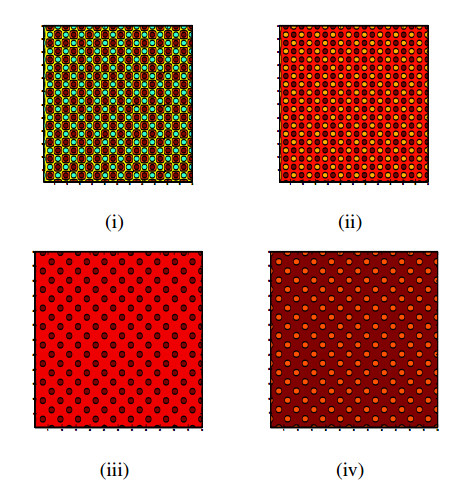
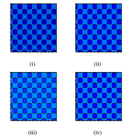
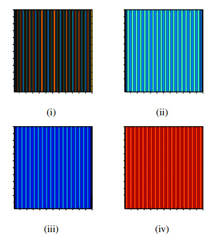
Incorporating self-diffusion and super-cross diffusion factors into the modeling approach enhances efficiency and realism by having a substantial impact on the scenario of pattern formation. Accordingly, this work analyzes self and super-cross diffusion for a predator-prey model. First, the stability of equilibrium points is explored. Utilizing stability analysis of local equilibrium points, we stabilize the properties that guarantee the emergence of the Turing instability. Weakly nonlinear analysis is used to get the amplitude equations at the Turing bifurcation point (WNA). The stability analysis of the amplitude equations establishes the conditions for the formation of small spots, hexagons, huge spots, squares, labyrinthine, and stripe patterns. Analytical findings have been validated using numerical simulations. Extensive data that may be used analytically and numerically to assess the effect of self-super-cross diffusion on a variety of predator-prey systems.

| [1] |
R. Arditi, L. R. Ginzburg, Coupling in predator-prey dynamics: ratio-dependence, J. Theor. Biol., 139 (1989), 311–326. https://doi.org/10.1016/S0022-5193(89)80211-5 doi: 10.1016/S0022-5193(89)80211-5

|
| [2] |
M. Banerjee, S. Abbas, Existence and non-existence of spatial patterns in a ratio-dependent predator-prey model, Ecol. Complex., 21 (2015), 199–214. https://doi.org/10.1016/j.ecocom.2014.05.005 doi: 10.1016/j.ecocom.2014.05.005
|
| [3] |
M. Banerjee, S. Ghorai, N. Mukherjee, Study of cross-diffusion induced Turing patterns in a ratio-dependent prey-predator model via amplitude equations, Appl. Math. Model., 55 (2018), 383–399. https://doi.org/10.1016/j.apm.2017.11.005 doi: 10.1016/j.apm.2017.11.005
|
| [4] |
M. Banerjee, N. Mukherjee, V. Volpert, Prey-predator model with a nonlocal bistable dynamics of prey, Mathematics, 6 (2018), 41. https://doi.org/10.3390/math6030041 doi: 10.3390/math6030041
|
| [5] |
M. A. Budroni, Cross-diffusion-driven hydrodynamic instabilities in a double-layer system: general classification and nonlinear simulations, Phys. Rev. E, 92 (2015), 063007. https://doi.org/10.1103/PhysRevE.92.063007 doi: 10.1103/PhysRevE.92.063007
|
| [6] |
M. Chen, R. Wu, L. Chen, Spatiotemporal patterns induced by Turing and Turing-Hopf bifurcations in a predator-prey system, Appl. Math. Comput., 380 (2020), 125300. https://doi.org/10.1016/j.amc.2020.125300 doi: 10.1016/j.amc.2020.125300
|
| [7] |
J. M. Chung, E. Peacock-Lopez, Cross-diffusion in the Templetor model of chemical self-replication, Phys. Lett. A, 371 (2007), 41–47. https://doi.org/10.1016/j.physleta.2007.04.114 doi: 10.1016/j.physleta.2007.04.114
|
| [8] |
S. M. Cox, P. C. Matthews, Exponential time differencing for stiff-systems, J. Comp. Phys., 176 (2002), 430–455. https://doi.org/10.1006/jcph.2002.6995 doi: 10.1006/jcph.2002.6995
|
| [9] |
M. C. Cross, P. C. Hohenberg, Pattern formation outside of equilibrium, Rev. Mod. Phys., 65 (1993), 851. https://doi.org/10.1103/RevModPhys.65.851 doi: 10.1103/RevModPhys.65.851
|
| [10] | H. I. Freedman, Deterministic mathematical models in population ecology, New York: Marcel Dekker Incorporated, 1980. |
| [11] |
P. Feng, Y. Kang, Dynamics of a modified Leslie-Gower model with double Allee effects, Nonlinear Dyn., 80 (2015), 1051–1062. https://doi.org/10.1007/s11071-015-1927-2 doi: 10.1007/s11071-015-1927-2
|
| [12] | G. Gambino, M. C. Lombardo, M. Sammartino, Pattern formation driven by cross–diffusion in a 2D domain, Nonlinear Anal. Real World Appl., 14 (2013), 1755–1779. |
| [13] | R. Gorenflo, F. Mainardi, Random walk models for space–fractional diffusion processes, Fract. Calc. Appl. Anal., 1 (1998), 167–191. |
| [14] |
G. Hu, X. Li, Y. Wang, Pattern formation and spatiotemporal chaos in a reaction-diffusion predator–prey system, Nonlinear Dyn., 81 (2015), 265–275. https://doi.org/10.1007/s11071-015-1988-2 doi: 10.1007/s11071-015-1988-2
|
| [15] |
N. Iqbal, R. Wu, B. Liu, Pattern formation by super–diffusion in FitzHugh–Nagumo model, Appl. Math. Comput., 313 (2017), 245–258. https://doi.org/10.1016/j.amc.2017.05.072 doi: 10.1016/j.amc.2017.05.072
|
| [16] |
N. Iqbal, Y. Karaca, Complex fractional-order HIV diffusion model based on amplitude equations with turing patterns and turing instability, Fractals, 29 (2021), 2140013. https://doi.org/10.1142/S0218348X21400132 doi: 10.1142/S0218348X21400132
|
| [17] |
N. Iqbal, R. Wu, W. W. Mohammed, Pattern formation induced by fractional cross-diffusion in a 3-species food chain model with harvesting, Math. Comput. Simul., 188 (2021), 102–119. https://doi.org/10.1016/j.matcom.2021.03.041 doi: 10.1016/j.matcom.2021.03.041
|
| [18] |
Y. Jia, P. Xue, Effects of the self- and cross-diffusion on positive steady states for a generalized predator-prey system, Nonlinear Anal. Real World Appl., 32 (2016), 229–241. https://doi.org/10.1016/j.nonrwa.2016.04.012 doi: 10.1016/j.nonrwa.2016.04.012
|
| [19] |
T. Kadota, K. Kuto, Positive steady states for a prey-predator model with some nonlinear diffusion terms, J. Math. Anal. Appl., 323 (2006), 1387–1401. https://doi.org/10.1016/j.jmaa.2005.11.065 doi: 10.1016/j.jmaa.2005.11.065
|
| [20] |
A. K. Kassam, L. N. Trefethen, Fourth-order time-stepping for stiff PDEs, SIAM J. Sci. Comp., 26 (2005), 1212–1233. https://doi.org/10.1137/S1064827502410633 doi: 10.1137/S1064827502410633
|
| [21] | E. Knobloch, J.D. Luca, Amplitude equations for travelling wave convection, Nonlinearity, 3 (1990), 975–980. |
| [22] |
K. Kuto, Y. Yamada, Multiple coexistence states for a prey-predator system with cross-diffusion, J. Differ. Eq., 197 (2004), 315–348. https://doi.org/10.1016/j.jde.2003.08.003 doi: 10.1016/j.jde.2003.08.003
|
| [23] |
B. Liu, R. Wu, N. Iqbal, L. Chen, Turing patterns in the Lengyel-Epstein system with superdiffusion, Int. J. Bifurcat. Chaos, 27 (2017), 1730026. https://doi.org/10.1142/S0218127417300269 doi: 10.1142/S0218127417300269
|
| [24] |
B. Liu, R. Wu, L. Chen, Patterns induced by super cross–diffusion in a predator-prey system with Michaelis-Menten type harvesting, Math. Biosci., 298 (2018), 71–79. https://doi.org/10.1016/j.mbs.2018.02.002 doi: 10.1016/j.mbs.2018.02.002
|
| [25] | J. D. Murray, Mathematical biology, Heidelberg: Springer, 1989. |
| [26] |
K. Oeda, Effect of cross-diffusion on the stationary problem of prey-predator model with a protection zone, J. Differ. Eq., 250 (2011), 3988–4009. https://doi.org/10.1016/j.jde.2011.01.026 doi: 10.1016/j.jde.2011.01.026
|
| [27] |
K. M. Owolabi, K. C. patidar, Numerical simulations for multicomponent ecological models with adaptive methods, Theor. Biol. Med. Model., 13 (2016), 1–25. https://doi.org/10.1186/s12976-016-0027-4 doi: 10.1186/s12976-016-0027-4
|
| [28] |
S. Pal, S. Ghorai, M. Banerjee, Analysis of a prey-predator model with non-local interaction in the prey population, Bull. Math. Biol., 80 (2018), 906–925. https://doi.org/10.1007/s11538-018-0410-x doi: 10.1007/s11538-018-0410-x
|
| [29] | S. G. Samko, A. A. Kilbas, O. I. Marichev, Fractional integrals and derivatives: theory and applications, New York: Gordon and Breach Science Publishers, 1993. |
| [30] |
N. Shigesada, K. Kawasaki, E. Teramoto, Spatial segregation of interacting species, J. Theor. Biol., 79 (1979), 83–99. https://doi.org/10.1016/0022-5193(79)90258-3 doi: 10.1016/0022-5193(79)90258-3
|
| [31] |
Y. L Song, R. Yang, G. Q Sun, Pattern dynamics in a Gierer-Meinhardt model with a saturating term, Appl. Math. Model., 46 (2017), 476–491. https://doi.org/10.1016/j.apm.2017.01.081 doi: 10.1016/j.apm.2017.01.081
|
| [32] |
C. Tian, L. Zhang, Z. Lin, Pattern formation for a model of plankton allelopathy with cross-diffusion, J. Franklin I., 348 (2011), 1947–1964. https://doi.org/10.1016/j.jfranklin.2011.05.013 doi: 10.1016/j.jfranklin.2011.05.013
|
| [33] |
C. M. Topaz, A. J. Catla, Forced patterns near a Turing-Hopf bifurcation, Phys. Rev. E, 81 (2010), 026213. https://doi.org/10.1103/PhysRevE.81.026213 doi: 10.1103/PhysRevE.81.026213
|
| [34] | L. N. Trefethen, Spectral methods in MATLAB, Philadelphia: SIAM Society for industrial and applied mathematics, 2000. |
| [35] |
M. A. Tsyganov, V. N. Biktashev, Classification of wave regimes in excitable systems with linear cross diffusion, Phys. Rev. E, 90 (2014), 062912. https://doi.org/10.1103/PhysRevE.90.062912 doi: 10.1103/PhysRevE.90.062912
|
| [36] | A. M. Turing, The chemical basis of morphogenesis, Phil. Trans. R. Soc. Lond. B, 237 (1952), 37–72. |
| [37] |
V. K. Vanag, I. R. Epstein, Cross-diffusion and pattern formation in reaction-diffusion systems, Phys. Chem. Chem. Phys., 11 (2009), 897–912. https://doi.org/10.1039/B813825G doi: 10.1039/B813825G
|
| [38] |
X. Ni, R. Yang, W. Wang, Y. Lai, C. Grebogi, Cyclic competition of mobile species on continuous space: Pattern formation and coexistence, Phys. Rev. E, 82 (2010), 066211. https://doi.org/10.1103/PhysRevE.82.066211 doi: 10.1103/PhysRevE.82.066211
|
| [39] |
S. Yuan, C. Xu, T. Zhang, Spatial dynamics in a predator-prey model with herd behavior, Chaos, 23 (2013), 033102. https://doi.org/10.1063/1.4812724 doi: 10.1063/1.4812724
|
| [40] |
E. P. Zemskov, K. Kassner, M. J. B. Hauser, W. Horsthemke, Turing space in reaction-diffusion systems with density-dependent cross diffusion, Phys. Rev. E, 87 (2013), 032906. https://doi.org/10.1103/PhysRevE.87.032906 doi: 10.1103/PhysRevE.87.032906
|
| [41] |
X. Zhang, G. Sun, Z. Jin, Spatial dynamics in a predator-prey model with Beddington-Deangelis functional response, Phys. Rev. E, 85 (2012), 021924. https://doi.org/10.1103/PhysRevE.85.021924 doi: 10.1103/PhysRevE.85.021924
|
| [42] |
T. Zhang, Y. Xing, H. Zang, M. Han, Spatio–temporal dynamics of a reaction–diffusion system for a predator–prey model with hyperbolic mortality, Nonlinear Dyn., 78 (2014), 265–277. https://doi.org/10.1007/s11071-014-1438-6 doi: 10.1007/s11071-014-1438-6
|
| [43] |
L. Zhang, C. R. Tian, Turing pattern dynamics in an activator-inhibitor system with super diffusion, Phys. Rev. E, 90 (2014), 062915. https://doi.org/10.1103/PhysRevE.90.062915 doi: 10.1103/PhysRevE.90.062915
|
Figures(7)

Naveed Iqbal, Ranchao Wu, Yeliz Karaca, Rasool Shah, Wajaree Weera. Pattern dynamics and Turing instability induced by self-super-cross-diffusive predator-prey model via amplitude equations[J]. AIMS Mathematics, 2023, 8(2): 2940-2960. doi: 10.3934/math.2023153


 DownLoad: