Theoretical and numerical aspects of the Malaria transmission model with piecewise technique

Shakeel Muhammad; Obaid J. Algahtani; Sayed Saifullah; Amir Ali; Shakeel Muhammad; Obaid J. Algahtani; Sayed Saifullah; Amir Ali

doi:10.3934/math.20231451

AIMS Mathematics

2023, Volume 8, Issue 12: 28353-28375. doi: 10.3934/math.20231451

Previous Article Next Article

Research article

Theoretical and numerical aspects of the Malaria transmission model with piecewise technique

1.
Department of Mathematics, University of Malakand, Chakdara, Dir(L), Khyber Pakhtunkhwa, Pakistan
2.
Department of Mathematics, College of Sciences, King Saud University, Riyadh 11451, Saudi Arabia

Received: 25 July 2023 Revised: 08 September 2023 Accepted: 27 September 2023 Published: 18 October 2023
MSC : 26A33, 34Axx, 34Lxx, 52Bxx, 65Yxx, 92-10

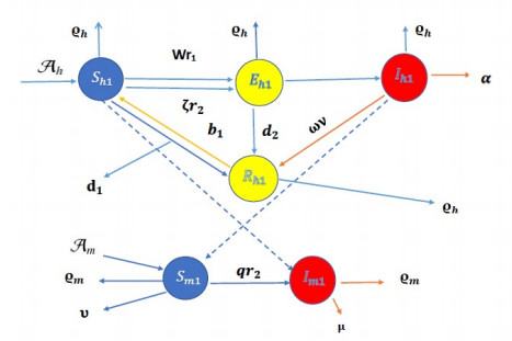
In this paper, we apply piecewise derivatives with both singular and non-singular kernels to investigate a malaria model. The singular kernel is the Caputo derivative, while the non-singular kernel is the Atangana-Baleanu operator in Caputo's sense (ABC). The existence, uniqueness, and numerical algorithm of the proposed model are presented using piecewise derivatives with both kernels. The stability is also presented for the proposed model using Ulam-Hyers stability. The numerical simulations are performed considering different fractional orders and compared the results with the real data to evaluate the efficiency of the proposed approach.
- piecewise operator,
- Caputo and Atangana-Baleanu operators,
- Malaria mathematical model
Citation: Shakeel Muhammad, Obaid J. Algahtani, Sayed Saifullah, Amir Ali. Theoretical and numerical aspects of the Malaria transmission model with piecewise technique[J]. AIMS Mathematics, 2023, 8(12): 28353-28375. doi: 10.3934/math.20231451

Related Papers:

Abstract

In this paper, we apply piecewise derivatives with both singular and non-singular kernels to investigate a malaria model. The singular kernel is the Caputo derivative, while the non-singular kernel is the Atangana-Baleanu operator in Caputo's sense (ABC). The existence, uniqueness, and numerical algorithm of the proposed model are presented using piecewise derivatives with both kernels. The stability is also presented for the proposed model using Ulam-Hyers stability. The numerical simulations are performed considering different fractional orders and compared the results with the real data to evaluate the efficiency of the proposed approach.

References

[1]	T. S. Faniran, A. O. Falade, J. Ogunsanwo, Sensitivity analysis of an untreated liver-stage Malaria, J. Comput. Sci. Comput. Math., 10 (2020), 61–68. https://doi.org/10.20967/jcscm.2020.04.002 doi: 10.20967/jcscm.2020.04.002
[2]	R. M. Anderson, R. M. May, Infectious diseases of humans: Dynamics and control, London: Oxford University Press, 1991.
[3]	L. Zhang, M. Rahman, M. Arfan, A. Ali, Investigation of mathematical model of transmission co-infection TB in HIV community with a non-singular kernel, Results Phys., 28 (2021), 104559. https://doi.org/10.1016/j.rinp.2021.104559 doi: 10.1016/j.rinp.2021.104559
[4]	Adnan, S. Ahmad, A. Ullah, M. B. Riaz, A. Ali, A. Akgül, et al., Complex dynamics of multi strain TB model under nonlocal and nonsingular fractal fractional operator, Results Phys., 30 (2021), 104823. https://doi.org/10.1016/j.rinp.2021.104823 doi: 10.1016/j.rinp.2021.104823
[5]	Adnan, A. Ali, M. Rahman, M. Arfan, Z. Shah, P. Kumam, W. Deebani, Investigation of time-fractional SIQR Covid-19 mathematical model with fractal-fractional Mittage-Leffler kernel, Alex. Eng. J., 61 (2022), 7771–7779. https://doi.org/10.1016/j.aej.2022.01.030 doi: 10.1016/j.aej.2022.01.030
[6]	C. J. Xu, S. Saifullah, A. Ali, Adnan, Theoretical and numerical aspects of Rubella disease model involving fractal fractional exponential decay kernel, Results Phys., 34 (2022), 105287. https://doi.org/10.1016/j.rinp.2022.105287 doi: 10.1016/j.rinp.2022.105287
[7]	A. Ullah, S. Ahmad, G. Rahman, A. Ali, F. Qayum, Agitation of SARS-CoV-2 disease (COVID-19) using ABC fractional-order modified SEIR model, Math. Methods Appl. Sci., 46 (2023), 12996–13011. https://doi.org/10.1002/mma.9229 doi: 10.1002/mma.9229
[8]	N. Ahmed, A. Elsonbaty, W. Adel, D. Baleanu, M. Rafiq, Stability analysis and numerical simulations of spatiotemporal HIV CD4+ T cell model with drug therapy, Chaos, 30 (2020), 083122. https://doi.org/10.1063/5.0010541 doi: 10.1063/5.0010541
[9]	W. Adel, A. Elsonbaty, A. Aldurayhim, A. El-Mesady, Investigating the dynamics of a novel fractional-order monkeypox epidemic model with optimal control, Alex. Eng. J., 73 (2023), 519–542. https://doi.org/10.1016/j.aej.2023.04.051 doi: 10.1016/j.aej.2023.04.051
[10]	A. El-Mesady, A. Elsonbaty, W. Adel, On nonlinear dynamics of a fractional order monkeypox virus model, Chaos Solitons Fractals, 164 (2022), 112716. https://doi.org/10.1016/j.chaos.2022.112716 doi: 10.1016/j.chaos.2022.112716
[11]	P. L. Li, Y. J. Lu, C. J. Xu, J. Ren, Insight into Hopf bifurcation and control methods in fractional order BAM neural networks incorporating symmetric structure and delay, Cogn. Comput., 2023. https://doi.org/10.1007/s12559-023-10155-2
[12]	D. Mu, C. Xu, Z. Liu, Y. Pang, Further insight into bifurcation and hybrid control tactics of a chlorine dioxide-iodine-malonic acid chemical reaction model incorporating delays, MATCH Commun. Math. Comput. Chem., 89 (2023), 529–566. http://doi.org/10.46793/match.89-3.529M doi: 10.46793/match.89-3.529M
[13]	E. A. Bakare, C. R. Nwozo, Mathematical analysis of the dynamics of Malaria disease transmission model, Int. J. Pure Appl. Math., 99 (2015), 411–437. http://doi.org/10.12732/ijpam.v99i4.3 doi: 10.12732/ijpam.v99i4.3
[14]	J. K. Baird, D. J. Fryauff, S. L. Hoffman, Primaquine for prevention of malaria in travelers, Clin. Infect. Dis., 37 (2003), 1659–1667. http://doi.org/10.1086/379714 doi: 10.1086/379714
[15]	M. Sinan, H. Ahmad, Z. Ahmad, J. Baili, S. Murtaza, M. A. Aiyashi, et al., Fractional mathematical modeling of malaria disease with treatment & insecticides, Results Phys., 34 (2022), 105220. https://doi.org/10.1016/j.rinp.2022.105220 doi: 10.1016/j.rinp.2022.105220
[16]	H. Y. Zhu, X. F. Zou, Dynamics of a HIV-1 infection model with cell-mediated immune response and intracellular delay, Discrete Contin. Dyn. Syst. Ser. S, 12 (2009), 511–524. https://doi.org/10.3934/dcdsb.2009.12.511 doi: 10.3934/dcdsb.2009.12.511
[17]	A. Atangana, D. Baleanu, New fractional derivatives with non-local and non-singular kernel: Theory and application to heat transfer model, Therm. Sci., 20 (2016), 763–769. https://doi.org/10.2298/TSCI160111018A doi: 10.2298/TSCI160111018A
[18]	A. Atangana, S. I. Araz, Nonlinear equations with global differential and integral operators: Existence, uniqueness with application to epidemiology, Results Phys., 20 (2020), 103593. http://doi.org/10.1016/j.rinp.2020.103593 doi: 10.1016/j.rinp.2020.103593
[19]	C. J. Xu, D. Mu, Y. L. Pan, C. Aouiti, L. Y. Yao, Exploring bifurcation in a fractional-order predator-prey system with mixed delays, J. Appl. Anal. Comput., 13 (2023), 1119–1136. https://doi.org/10.11948/20210313 doi: 10.11948/20210313
[20]	C. J. Xu, D. Mu, Z. X. Liu, Y. C. Pang, C. Aouiti, O. Tunc, et al., Bifurcation dynamics and control mechanism of a fractional-order delayed Brusselator chemical reaction model, MATCH Commun. Math. Comput. Chem., 89 (2023), 73–106. https://doi.org/10.46793/match.89-1.073X doi: 10.46793/match.89-1.073X
[21]	C. J. Xu, X. H. Cui, P. L. Li, J. L. Yan, L. Y. Yao, Exploration on dynamics in a discrete predator-prey competitive model involving time delays and feedback controls, J. Biol. Dyn., 17 (2023), 2220349. https://doi.org/10.1080/17513758.2023.2220349 doi: 10.1080/17513758.2023.2220349
[22]	C. J. Xu, Q. Y. Cui, Z. X. Liu, Y. L. Pan, X. H. Cui, W. Ou, et al., Extended hybrid controller design of bifurcation in a delayed chemostat model, MATCH Commun. Math. Comput. Chem., 90 (2023), 609–648. https://doi.org/10.46793/match.90-3.609X doi: 10.46793/match.90-3.609X
[23]	A. Atangana, S. I. Araz, Mathematical model of COVID-19 spread in Turkey and South Africa: Theory, methods and applications, Adv. Differ. Equ., 2020 (2020), 1–87. https://doi.org/10.1101/2020.05.08.20095588 doi: 10.1101/2020.05.08.20095588
[24]	A. Atangana, S. I. Araz, New concept in calculus: Piecewise differential and integral operators, Chaos Soliton. Fract., 145 (2021), 110638. https://doi.org/10.1016/j.chaos.2020.110638 doi: 10.1016/j.chaos.2020.110638
[25]	S. Saifullah, S. Ahmad, F. Jarad, Study on the dynamics of a piecewise tumor-immune interaction model, Fractals, 30 (2022), 2240233. https://doi.org/10.1142/S0218348X22402332 doi: 10.1142/S0218348X22402332
[26]	S. Ahmad, M. F. Yassen, M. M. Alam, S. Alkhati, F. Jarad, M. B. Riaz, A numerical study of dengue internal transmission model with fractional piecewise derivative, Results Phys., 39 (2022), 105798. https://doi.org/10.1016/j.rinp.2022.105798 doi: 10.1016/j.rinp.2022.105798
[27]	H. D. Qu, S. Saifullah, J. Khan, A. Khan, M. Rahman, G. D. Zheng, Dynamics of leptospirosis disease in context of piecewise classical-global and classical-fractional operators, Fractals, 30 (2022), 2240216. https://doi.org/10.1142/S0218348X22402162 doi: 10.1142/S0218348X22402162
[28]	A. Ali, S. Althobaiti, A. Althobaiti, K. Khan, R. Jan, Chaotic dynamics in a non-linear tumor-immune model with Caputo-Fabrizio fractional operator, Eur. Phys. J. Spec. Top., 2023. https://doi.org/10.1140/epjs/s11734-023-00929-y
[29]	R. P. Kellogg, Uniqueness in the Schauder fixed point theorem, Proc. Amer. Math. Soc., 60 (1976), 207–210.
[30]	R. S. Palais, A simple proof of the Banach contraction principle, J. Fixed Point Theory Appl., 2 (2007), 221–223. https://doi.org/10.1007/s11784-007-0041-6 doi: 10.1007/s11784-007-0041-6
[31]	World Health Organization, Estimated number of malaria cases, 2023. Available from: https://www.who.int/data/gho/data/indicators/indicator-details/GHO/estimated-number-of-malaria-cases

Reader Comments

Your name:*

Email:*
© 2023 the Author(s), licensee AIMS Press. This is an open access article distributed under the terms of the Creative Commons Attribution License (http://creativecommons.org/licenses/by/4.0)