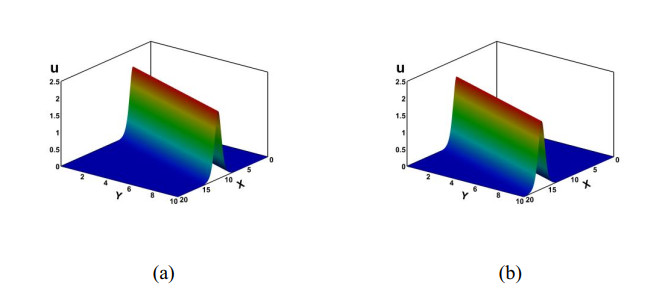
Recently, considerable attention has been given to (2+1)-dimensional Kadomtsev-Petviashvili equations due to their extensive applications in solitons that widely exist in nonlinear science. Therefore, developing a reliable numerical algorithm for the Kadomtsev-Petviashvili equations is crucial. The lattice Boltzmann method, which has been an efficient simulation method in the last three decades, is a promising technique for solving Kadomtsev-Petviashvili equations. However, the traditional higher-order moment lattice Boltzmann model for the Kadomtsev-Petviashvili equations suffers from low accuracy because of error accumulation. To overcome this shortcoming, a splitting lattice Boltzmann scheme for (2+1)-dimensional Kadomtsev-Petviashvili-Ⅰ type equations is proposed in this paper. The variable substitution method is applied to transform the Kadomtsev-Petviashvili-Ⅰ type equation into two macroscopic equations. Two sets of distribution functions are employed to construct these two macroscopic equations. Moreover, three types of soliton solutions are numerically simulated by this algorithm. The numerical results imply that the splitting lattice Boltzmann schemes have an advantage over the traditional high-order moment lattice Boltzmann model in simulating the Kadomtsev-Petviashvili-Ⅰ type equations.
Citation: Boyu Wang. A splitting lattice Boltzmann scheme for (2+1)-dimensional soliton solutions of the Kadomtsev-Petviashvili equation[J]. AIMS Mathematics, 2023, 8(11): 28071-28089. doi: 10.3934/math.20231436
Recently, considerable attention has been given to (2+1)-dimensional Kadomtsev-Petviashvili equations due to their extensive applications in solitons that widely exist in nonlinear science. Therefore, developing a reliable numerical algorithm for the Kadomtsev-Petviashvili equations is crucial. The lattice Boltzmann method, which has been an efficient simulation method in the last three decades, is a promising technique for solving Kadomtsev-Petviashvili equations. However, the traditional higher-order moment lattice Boltzmann model for the Kadomtsev-Petviashvili equations suffers from low accuracy because of error accumulation. To overcome this shortcoming, a splitting lattice Boltzmann scheme for (2+1)-dimensional Kadomtsev-Petviashvili-Ⅰ type equations is proposed in this paper. The variable substitution method is applied to transform the Kadomtsev-Petviashvili-Ⅰ type equation into two macroscopic equations. Two sets of distribution functions are employed to construct these two macroscopic equations. Moreover, three types of soliton solutions are numerically simulated by this algorithm. The numerical results imply that the splitting lattice Boltzmann schemes have an advantage over the traditional high-order moment lattice Boltzmann model in simulating the Kadomtsev-Petviashvili-Ⅰ type equations.

| [1] |
S. Chen, H. Chen, D. Martínez, W. Matthaeus, Lattice Boltzmann model for simulation of magneto-hydrodynamics, Phys. Rev. Lett., 67 (1991), 3776–3779. https://doi.org/10.1103/PhysRevLett.67.3776 doi: 10.1103/PhysRevLett.67.3776

|
| [2] |
R. Benzi, S. Succi, M. Vergassola, The lattice Boltzmann equation: theory and applications, Phys. Rep., 222 (1992), 145–197. https://doi.org/10.1016/0370-1573(92)90090-M doi: 10.1016/0370-1573(92)90090-M
|
| [3] |
Y. H. Qian, D. d'Humières, P. Lallemand, Lattice BGK models for Navier-Stokes equation, Europhys. Lett., 17 (1992), 479–484. https://doi.org/10.1209/0295-5075/17/6/001 doi: 10.1209/0295-5075/17/6/001
|
| [4] |
A. Fakhari, M. Geier, T. Lee, A mass-conserving lattice Boltzmann method with dynamic grid refinement for immiscible two-phase flows, J. Comput. Phys., 315 (2016), 434–457. https://doi.org/10.1016/j.jcp.2016.03.058 doi: 10.1016/j.jcp.2016.03.058
|
| [5] |
T. Reis, A lattice Boltzmann formulation of the one-fluid model for multiphase flow, J. Comput. Phys., 453 (2022), 110962. https://doi.org/10.1016/j.jcp.2022.110962 doi: 10.1016/j.jcp.2022.110962
|
| [6] |
Q. Z. Li, Z. L. Lu, Z. Chen, C. Shu, Y. Y. Liu, T. Q. Guo, et al., An efficient simplified phase-field lattice Boltzmann method for super-large-density-ratio multiphase flow, Int. J. Multiph. Flow, 160 (2023), 104368. https://doi.org/10.1016/j.ijmultiphaseflow.2022.104368 doi: 10.1016/j.ijmultiphaseflow.2022.104368
|
| [7] | S. Simonis, J. Nguyen, S. J. Avis, W. Dörfler, M. J. Krause, Binary fluid flow simulations with free energy lattice Boltzmann methods, Discrete Cont. Dyn. S, in press, 2023. http://doi.org/10.3934/dcdss.2023069 |
| [8] |
F. Bukreev, S. Simonis, A. Kummerlӓnder, J. Jeßberger, M. J. Krause, Consistent lattice Boltzmann methods for the volume averaged Navier-Stokes equations, J. Comput. Phys., 490 (2023), 112301. https://doi.org/10.1016/j.jcp.2023.112301 doi: 10.1016/j.jcp.2023.112301
|
| [9] |
M. H. Saadat, F. Bösch, I. V. Karlin, Lattice Boltzmann model for compressible flows on standard lattices: Variable Prandtl number and adiabatic exponent, Phys. Rev. E, 99 (2019), 013306. https://doi.org/10.1103/PhysRevE.99.013306 doi: 10.1103/PhysRevE.99.013306
|
| [10] |
X. Zhao, L. Yang, C. Shu, An implicit lattice Boltzmann flux solver for simulation of compressible flows, Comput. Math. Appl., 107 (2022), 82–94. https://doi.org/10.1016/j.camwa.2021.12.014 doi: 10.1016/j.camwa.2021.12.014
|
| [11] |
K. Suga, Y. Kuwata, K. Takashima, R. Chikasue, A D3Q27 multiple-relaxation-time lattice Boltzmann method for turbulent flows, Comput. Math. Appl., 69 (2015), 518–529. https://doi.org/10.1016/j.camwa.2015.01.010 doi: 10.1016/j.camwa.2015.01.010
|
| [12] |
M. Taha, S. Zhao, A. Lamorlette, J. L. Consalvi, P. Boivin, Lattice-Boltzmann modeling of buoyancy-driven turbulent flows, Phys. Fluids, 34 (2022), 055131. https://doi.org/10.1063/5.0088409 doi: 10.1063/5.0088409
|
| [13] |
S. Chen, Z. Liu, C. Zhang, Z. He, Z. W. Tian, B. C. Shi, et al., A novel coupled lattice Boltzmann model for low Mach number combustion simulation, Appl. Math. Comput., 193 (2007), 266–284. https://doi.org/10.1016/j.amc.2007.03.087 doi: 10.1016/j.amc.2007.03.087
|
| [14] |
K. Bhairapurada, B. Denet, P. Boivin, A Lattice-Boltzmann study of premixed flames thermo-acoustic instabilities, Combust. Flame, 240 (2022), 112049. https://doi.org/10.1016/j.combustflame.2022.112049 doi: 10.1016/j.combustflame.2022.112049
|
| [15] |
Z. Chen, C. Shu, Simplified lattice Boltzmann method for non-Newtonian power-law fluid flows, Int. J. Numer. Methods Fluids, 92 (2019), 38–54. https://doi.org/10.1002/fld.4771 doi: 10.1002/fld.4771
|
| [16] |
S. Adam, F. Hajabdollahi, K. N. Premnath, Cascaded lattice Boltzmann modeling and simulations of three-dimensional non-Newtonian fluid flows, Comput. Phys. Commun., 262 (2021), 107858. https://doi.org/10.1016/j.cpc.2021.107858 doi: 10.1016/j.cpc.2021.107858
|
| [17] |
G. Yan, A lattice Boltzmann equation for waves, J. Comput. Phys., 161 (2000), 61–69. https://doi.org/10.1006/jcph.2000.6486 doi: 10.1006/jcph.2000.6486
|
| [18] |
A. M. Velasco, J. D. Muñoz, M. Mendoza, Lattice Boltzmann model for the simulation of the wave equation in curvilinear coordinates, J. Comput. Phys., 376 (2019), 76–97. https://doi.org/10.1016/j.jcp.2018.09.031 doi: 10.1016/j.jcp.2018.09.031
|
| [19] |
D. Li, H. Lai, B. Shi, Mesoscopic simulation of the (2+1)-dimensional wave equation with nonlinear damping and source terms using the lattice Boltzmann BGK model, Entropy, 21 (2019), 390. https://doi.org/10.3390/e21040390 doi: 10.3390/e21040390
|
| [20] |
G. Yan, J. Zhang, A higher-order moment method of the lattice Boltzmann model for the Korteweg-de Vries equation, Math. Comput. Simul., 79 (2009), 1554–1565. https://doi.org/10.1016/j.matcom.2008.07.006 doi: 10.1016/j.matcom.2008.07.006
|
| [21] |
H. Wang, Solitary wave of the Korteweg-de Vries equation based on lattice Boltzmann model with three conservation laws, Adv. Space Res., 59 (2017), 283–292. https://doi.org/10.1016/j.asr.2016.08.023 doi: 10.1016/j.asr.2016.08.023
|
| [22] |
W. Q. Hu, S. L. Jia, General propagation lattice Boltzmann model for variable-coefficient non-isospectral KdV equation, Appl. Math. Lett., 91 (2019), 61–67. https://doi.org/10.1016/j.aml.2018.12.002 doi: 10.1016/j.aml.2018.12.002
|
| [23] |
H. Yoshida, M. Nagaoka, Lattice Boltzmann method for the convection-diffusion equation in curvilinear coordinate systems, J. Comput. Phys., 257 (2014), 884–900. https://doi.org/10.1016/j.jcp.2013.09.035 doi: 10.1016/j.jcp.2013.09.035
|
| [24] |
L. Wang, B. Shi, Z. Chai, Regularized lattice Boltzmann model for a class of convection-diffusion equations, Phys. Rev. E, 92 (2015), 043311. https://doi.org/10.1103/PhysRevE.92.043311 doi: 10.1103/PhysRevE.92.043311
|
| [25] |
Z. Chai, B. Shi, Z. Guo, A multiple-relaxation-time lattice Boltzmann model for general nonlinear anisotropic convection-diffusion equations, J. Sci. Comput., 69 (2016), 355–390. https://doi.org/10.1007/s10915-016-0198-5 doi: 10.1007/s10915-016-0198-5
|
| [26] |
J. Zhang, G. Yan, A lattice Boltzmann model for reaction-diffusion equations with higher-order accuracy, J. Sci. Comput., 52 (2012), 1–16. https://doi.org/10.1007/s10915-011-9530-2 doi: 10.1007/s10915-011-9530-2
|
| [27] |
G. Silva, Discrete effects on the source term for the lattice Boltzmann modelling of one-dimensional reaction-diffusion equations, Comput. Fluids, 251 (2023), 105735. https://doi.org/10.1016/j.compfluid.2022.105735 doi: 10.1016/j.compfluid.2022.105735
|
| [28] |
L. Zhong, S. Feng, P. Dong, S. T. Gao, Lattice Boltzmann schemes for the nonlinear Schrödinger equation, Phys. Rev. E, 74 (2006), 036704. https://doi.org/10.1103/PhysRevE.74.036704 doi: 10.1103/PhysRevE.74.036704
|
| [29] |
B. Wang, J. Zhang, G. Yan, Curvilinear coordinate lattice Boltzmann simulation for necklace-ring beams in the nonlinear Schrödinger equation, Int. J. Mod. Phys. C, 31 (2020), 2050136. https://doi.org/10.1142/S0129183120501363 doi: 10.1142/S0129183120501363
|
| [30] | B. B. Kadomtsev, V. I. Petviashvili, On the stability of solitary waves in weakly dispersive media, Sov. Phys. Dokl., 15 (1970), 175–187. |
| [31] |
P. J. Bryant, Two-dimensional periodic permanent waves in shallow water, J. Fluid Mech., 115 (1982), 525–532. https://doi.org/10.1017/S0022112082000895 doi: 10.1017/S0022112082000895
|
| [32] |
J. Hammack, N. Scheffner, H. Segur, Two-dimensional periodic waves in shallow water, J. Fluid Mech., 209 (1989), 567–589. https://doi.org/10.1017/S0022112089003228 doi: 10.1017/S0022112089003228
|
| [33] |
J. K. Xue, A spherical KP equation for dust acoustic waves, Phys. Lett. A, 314 (2003), 479–483. https://doi.org/10.1016/S0375-9601(03)00951-4 doi: 10.1016/S0375-9601(03)00951-4
|
| [34] |
I. M. Krichever, S. P. Novikov, Holomorphic bundles over algebraic curves and nonlinear equations, Russ. Math. Surv., 35 (1980), 53–64. https://doi.org/10.1070/RM1980v035n06ABEH001974 doi: 10.1070/RM1980v035n06ABEH001974
|
| [35] |
G. A. Latham, Solutions of the KP equation associated to rank-three commuting differential operators over a singular elliptic curve, Physica D, 41 (1990), 55–66. https://doi.org/10.1016/0167-2789(90)90027-M doi: 10.1016/0167-2789(90)90027-M
|
| [36] |
H. Zhao, Interactions of solitary waves under the conditions of the (3+1)-dimensional Kadomtsev-Petviashvili equation, Appl. Math. Comput., 215 (2010), 3383–3389. https://doi.org/10.1016/j.amc.2009.10.031 doi: 10.1016/j.amc.2009.10.031
|
| [37] |
C. Y. Qin, S. F. Tian, X. B. Wang, T. T. Zhang, J. Li, Rogue waves, bright–dark solitons and traveling wave solutions of the (3+1)-dimensional generalized Kadomtsev-Petviashvili equation, Comput. Math. Appl., 75 (2018), 4221–4231. https://doi.org/10.1016/j.camwa.2018.03.024 doi: 10.1016/j.camwa.2018.03.024
|
| [38] |
L. Li, Y. Xie, M. Wang, Characteristics of the interaction behavior between solitons in (2+1)-dimensional caudrey-dodd-gibbon-kotera-sawada equation, Results Phys., 19 (2020), 103697. https://doi.org/10.1016/j.rinp.2020.103697 doi: 10.1016/j.rinp.2020.103697
|
| [39] |
J. G. Liu, W. H. Zhu, Y. K. Wu, G. H. Jin, Application of multivariate bilinear neural network method to fractional partial differential equations, Results Phys., 47 (2023), 106341. https://doi.org/10.1016/j.rinp.2023.106341 doi: 10.1016/j.rinp.2023.106341
|
| [40] |
J. G. Liu, M. Eslami, H. Rezazadeh, M. Mirzazadeh, Rational solutions and lump solutions to a non-isospectral and generalized variable-coefficient Kadomtsev-Petviashvili equation, Nonlinear Dyn., 95 (2019), 1027–1033. https://doi.org/10.1007/s11071-018-4612-4 doi: 10.1007/s11071-018-4612-4
|
| [41] |
J. G. Liu, Q. Ye, Stripe solitons and lump solutions for a generalized Kadomtsev–Petviashvili equation with variable coefficients in fluid mechanics, Nonlinear Dyn., 96 (2019), 23–29. https://doi.org/10.1007/s11071-019-04770-8 doi: 10.1007/s11071-019-04770-8
|
| [42] |
L. Li, Y. Xie, L. Mei, Multiple-order rogue waves for the generalized (2+1)-dimensional Kadomtsev-Petviashvili equation, Appl. Math. Lett., 117 (2021), 107079. https://doi.org/10.1016/j.aml.2021.107079 doi: 10.1016/j.aml.2021.107079
|
| [43] |
L. Li, Y. Xie, Rogue wave solutions of the generalized (3+1)-dimensional Kadomtsev-Petviashvili equation, Chaos Soliton Fract., 147 (2021), 110935. https://doi.org/10.1016/j.chaos.2021.110935 doi: 10.1016/j.chaos.2021.110935
|
| [44] |
Y. Xie, Y. Yan, L. Li, Rational solutions and rogue waves of the generalized (2+1)-dimensional Kadomtsev-Petviashvili equation, Chinese J. Phys., 77 (2022), 2047–2059. https://doi.org/10.1016/j.cjph.2021.11.010 doi: 10.1016/j.cjph.2021.11.010
|
| [45] |
J. G. Liu, W. H. Zhu, Y. He, Variable-coefficient symbolic computation approach for finding multiple rogue wave solutions of nonlinear system with variable coefficients, Z. Angew. Math. Phys., 72 (2021), 154. https://doi.org/10.1007/s00033-021-01584-w doi: 10.1007/s00033-021-01584-w
|
| [46] |
A. R. Seadawy, K. El-Rashidy, Dispersive solitary wave solutions of Kadomtsev-Petviashvili and modified Kadomtsev-Petviashvili dynamical equations in unmagnetized dust plasma, Results Phys., 8 (2018), 1216–1222. https://doi.org/10.1016/j.rinp.2018.01.053 doi: 10.1016/j.rinp.2018.01.053
|
| [47] |
A. G. Bratsos, E. H. Twizell, An explicit finite difference scheme for the solution of Kadomtsev-Petviashvili equation, Int. J. Comput. Math., 68 (1998), 175–187. https://doi.org/10.1080/00207169808804685 doi: 10.1080/00207169808804685
|
| [48] |
B. F. Feng, T. Mitsui, A finite difference method for the Korteweg-de Vries and the Kadomtsev-Petviashvili equations, J. Comput. Appl. Math., 90 (1998), 95–116. https://doi.org/10.1016/S0377-0427(98)00006-5 doi: 10.1016/S0377-0427(98)00006-5
|
| [49] |
A. A. Minzoni, N. F. Smyth, Evolution of lump solutions for the KP equation, Wave Motion, 24 (1996), 291–305. https://doi.org/10.1016/S0165-2125(96)00023-6 doi: 10.1016/S0165-2125(96)00023-6
|
| [50] |
A. M. Wazwaz, A computational approach to soliton solutions of the Kadomtsev-Petviashvili equation, Appl. Math. Comput., 123 (2001), 205–217. https://doi.org/10.1016/S0096-3003(00)00065-5 doi: 10.1016/S0096-3003(00)00065-5
|
| [51] |
H. M. Wang, Solitons of the Kadomtsev-Petviashvili equation based on lattice Boltzmann model, Adv. Space Res., 59 (2017), 293–301. https://doi.org/10.1016/j.asr.2016.08.029 doi: 10.1016/j.asr.2016.08.029
|
| [52] | J. Cai, J. Chen, M. Chen, Efficient linearized local energy-preserving method for the Kadomtsev-Petviashvili equation, Discrete Cont. Dyn. B, 27 (2022), 2441–2453. |
| [53] | S. Beji, Kadomtsev-Petviashvili type equation for uneven water depths, Ocean Eng., 154 (2018), 226–233. |
| [54] |
B. Fornberg, G. B. Whitham, A numerical and theoretical study of certain nonlinear wave phenomena, Philos. Trans. Roy. Soc. A, 289 (1978), 373–403. https://doi.org/10.1098/rsta.1978.0064 doi: 10.1098/rsta.1978.0064
|
| [55] | S. Chapman, T. G. Cowling, The Mathematical Theory of Non-Uniform Gases, Cambridge: Cambridge University Press, 1970. |
| [56] |
S. Hou, Q. Zhou, S. Chen, G. Doolen, A. C. Cogley, Simulation of cavity flow by the lattice Boltzmann method, J. Comput. Phys., 118 (1995), 329–347. https://doi.org/10.1006/jcph.1995.1103 doi: 10.1006/jcph.1995.1103
|


Figures(5) / Tables(1)

Boyu Wang. A splitting lattice Boltzmann scheme for (2+1)-dimensional soliton solutions of the Kadomtsev-Petviashvili equation[J]. AIMS Mathematics, 2023, 8(11): 28071-28089. doi: 10.3934/math.20231436


 DownLoad: