Numerical simulation for the fractional-in-space Ginzburg-Landau equation using Fourier spectral method

Xiao-Yu Li; Yu-Lan Wang; Zhi-Yuan Li; Xiao-Yu Li; Yu-Lan Wang; Zhi-Yuan Li

doi:10.3934/math.2023124

AIMS Mathematics

2023, Volume 8, Issue 1: 2407-2418. doi: 10.3934/math.2023124

Previous Article Next Article

Research article

Numerical simulation for the fractional-in-space Ginzburg-Landau equation using Fourier spectral method

1.
Department of Mathematics, Inner Mongolia University of Technology, Hohhot, 010051, China
2.
College of Date Science and Application, Inner Mongolia University of Technology, Hohhot, 010080, China

Received: 02 August 2022 Revised: 19 September 2022 Accepted: 26 September 2022 Published: 02 November 2022
MSC : 78M22, 81Q05

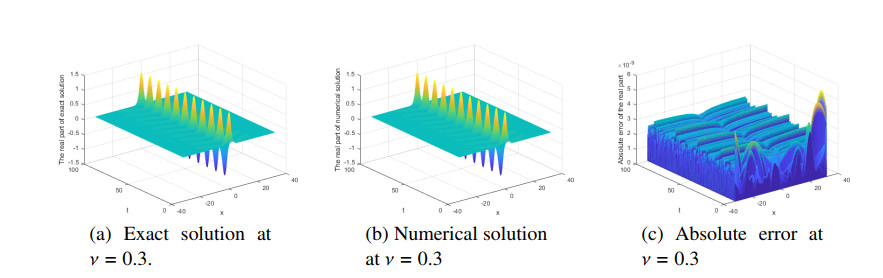
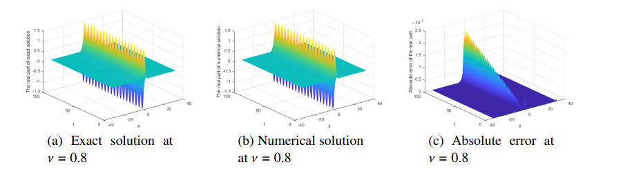
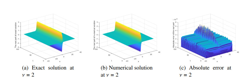
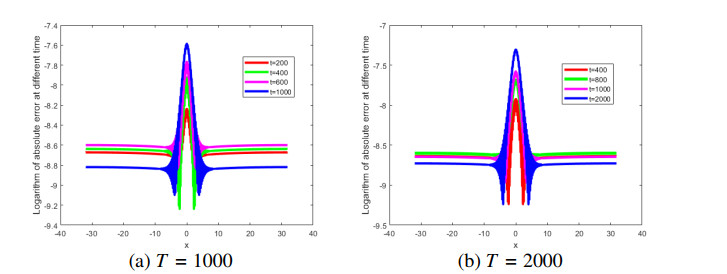
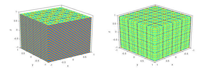
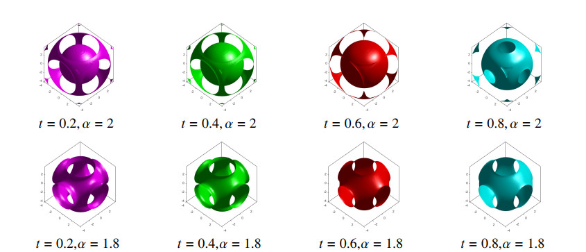
This paper uses the Fourier spectral method to study the propagation and interaction behavior of the fractional-in-space Ginzburg-Landau equation in different parameters and different fractional derivatives. Comparisons are made between the numerical and the exact solution, and it is found that the Fourier spectral method is a satisfactory and efficient algorithm for capturing the propagation of the fractional-in-space Ginzburg-Landau equation. Experimental findings indicate that the proposed method is easy to implement, effective and convenient in the long-time simulation for solving the proposed model. The influence of the fractional Laplacian operator on the fractional-in-space Ginzburg-Landau equation and some of the propagation behaviors of the 3D fractional-in-space Ginzburg-Landau equation are observed. In Experiment 2, we observe the propagation behaviors of the 3D fractional-in-space Ginzburg-Landau equation which are unlike any that have been previously obtained in numerical studies.
- fractional Ginzburg-Landau equation,
- Laplacian operator,
- Fourier spectral method,
- numerical simulation
Citation: Xiao-Yu Li, Yu-Lan Wang, Zhi-Yuan Li. Numerical simulation for the fractional-in-space Ginzburg-Landau equation using Fourier spectral method[J]. AIMS Mathematics, 2023, 8(1): 2407-2418. doi: 10.3934/math.2023124

Related Papers:

Abstract

This paper uses the Fourier spectral method to study the propagation and interaction behavior of the fractional-in-space Ginzburg-Landau equation in different parameters and different fractional derivatives. Comparisons are made between the numerical and the exact solution, and it is found that the Fourier spectral method is a satisfactory and efficient algorithm for capturing the propagation of the fractional-in-space Ginzburg-Landau equation. Experimental findings indicate that the proposed method is easy to implement, effective and convenient in the long-time simulation for solving the proposed model. The influence of the fractional Laplacian operator on the fractional-in-space Ginzburg-Landau equation and some of the propagation behaviors of the 3D fractional-in-space Ginzburg-Landau equation are observed. In Experiment 2, we observe the propagation behaviors of the 3D fractional-in-space Ginzburg-Landau equation which are unlike any that have been previously obtained in numerical studies.

References

[1]	I. S. Aranson, L. Kramer, The world of the complex Ginzburg-Landau equation, Rev. Mod. Phys., 74 (2002), 99–143. https://doi.org/10.1103/RevModPhys.74.99 doi: 10.1103/RevModPhys.74.99
[2]	A. Atangana, R. T. Alqahtani, New numerical method and application to Keller-Segel model with fractional order derivative, Chaos Soliton. Fract., 116 (2018), 14–21. https://doi.org/10.1016/j.chaos.2018.09.013 doi: 10.1016/j.chaos.2018.09.013
[3]	K. M. Owolabi, A. Atangana, Numerical methods for fractional differentiation, Singapore: Springer, 2019. https://doi.org/10.1007/978-981-15-0098-5
[4]	S. Ahmad, S. Javeed, H. Ahmad, J. Khushi, S. K. Elagan, A. Khames, Analysis and numerical solution of novel fractional model for dengue, Results Phys., 28 (2021), 104669. https://doi.org/10.1016/j.rinp.2021.104669 doi: 10.1016/j.rinp.2021.104669
[5]	Z. U. Zafar, S. Zaib, M. T. Hussain, C. Tunç, S. Javeed, Analysis and numerical simulation of tuberculosis model using different different fractional derivatives, Chaos Soliton. Fract., 160 (2022), 112202. https://doi.org/10.1016/j.chaos.2022.112202 doi: 10.1016/j.chaos.2022.112202
[6]	I. Podlubny, Fractional differential equations: An introduction to fractional derivatives, fractional differential equations to methods of their solution and some of their applications, San Diego: Academic Press, 1999.
[7]	X. Y. Li, C. Han, Y. L. Wang, Novel patterns in fractional-in-space nonlinear coupled FitzHugh-Nagumo models with Riesz fractional derivative, Fractal Fract., 6 (2022), 136. https://doi.org/10.3390/fractalfract6030136 doi: 10.3390/fractalfract6030136
[8]	V. E. Tarasov, G. M. Zaslavsky, Fractional Ginzburg-Landau equation for fractal media, Physica A, 354 (2005), 249–261. https://doi.org/10.1016/j.physa.2005.02.047 doi: 10.1016/j.physa.2005.02.047
[9]	V. E. Tarasov, G. M. Zaslavsky, Fractional dynamics of coupled oscillators with long-range interaction, Chaos, 16 (2006), 023110. https://doi.org/10.1063/1.2197167 doi: 10.1063/1.2197167
[10]	M. D. Ortigueira, T. M. Laleg-Kirati, J. A. T. Machado, Riesz potential versus fractional Laplacian, J. Statis. Mech., 2014 (2014), P09032. https://doi.org/10.1088/1742-5468/2014/09/P09032 doi: 10.1088/1742-5468/2014/09/P09032
[11]	Q. F. Zhang, L. Zhang, H. W. Sun, A three-level finite difference method with preconditioning technique for two-dimensional nonlinear fractional complex Ginzburg-Landau equations, J. Comput. Appl. Math., 389 (2021), 113355. https://doi.org/10.1016/j.cam.2020.113355 doi: 10.1016/j.cam.2020.113355
[12]	M. Zhang, G. F. Zhang, L. D. Liao, Fast iterative solvers and simulation for the space fractional Ginzburg-Landau equations, Comput. Math. Appl., 78 (2019), 1793–1800. https://doi.org/10.1016/j.camwa.2019.01.026 doi: 10.1016/j.camwa.2019.01.026
[13]	R. Du, Y. Y. Wang, Z. P. Hao, High-dimensional nonlinear Ginzburg-Landau equation with fractional Laplacian: Discretization and simulations, Commun. Nonlinear Sci., 102 (2021), 105920. https://doi.org/10.1016/j.cnsns.2021.105920 doi: 10.1016/j.cnsns.2021.105920
[14]	P. D. Wang, Fast exponential time differencing/spectral-Galerkin method for the nonlinear fractional Ginzburg-Landau equation with fractional Laplacian in unbounded domain, Appl. Math. Lett., 112 (2021), 106710. https://doi.org/10.1016/j.aml.2020.106710 doi: 10.1016/j.aml.2020.106710
[15]	M. Li, C. M. Huang, N. Wang, Galerkin finite element method for the nonlinear fractional Ginzburg-Landau equation, Appl. Numer. Math., 118 (2017), 131–149. https://doi.org/10.1016/j.apnum.2017.03.003 doi: 10.1016/j.apnum.2017.03.003
[16]	N. Akhmediev, V. Afanasjev, J. Soto-Crespo, Singularities and special soliton solutions of the cubic-quintic complex Ginzburg-Landau equation, Phys. Rev. E, 53 (1996), 1190. https://doi.org/10.1103/PhysRevE.53.1190 doi: 10.1103/PhysRevE.53.1190
[17]	C. Han, Y. L. Wang, Numerical solutions of variable-coefficient fractional-in-space KdV equation with the Caputo fractional derivative, Fractal Fract., 6 (2022), 207. https://doi.org/10.3390/fractalfract6040207 doi: 10.3390/fractalfract6040207
[18]	C. Han, Y. L. Wang, Z. Y. Li, A high-precision numerical approach to solving space fractional Gray-Scott model, Appl. Math. Lett., 125 (2022), 107759. https://doi.org/10.1016/j.aml.2021.107759 doi: 10.1016/j.aml.2021.107759

Reader Comments

Your name:*

Email:*
© 2023 the Author(s), licensee AIMS Press. This is an open access article distributed under the terms of the Creative Commons Attribution License (http://creativecommons.org/licenses/by/4.0)