Dynamical complexities and chaos control in a Ricker type predator-prey model with additive Allee effect

1.   Introduction

In recent years, human beings have been faced with the problem of resource shortage and environmental deterioration. Therefore, more and more people are interested in the analysis of predator-prey bio-economic systems. The authors proposed a singular bio-economic system with the invasion alien species in ^[1]. The stability and sliding mode control of a single bio-economic system was analyzed in ^[2]. The fuzzy stochastic optimal guaranteed cost control of bio-economic singular Markovian jump systems (MJSs) was studied in ^[3]. A singular bio-economic MJS with commodity prices as Markov chains was proposed in ^[4]. The exponential stability in mean square for MJSs was discussed in ^[31]. The problem of bifurcation and control for the biological economic system had been considered in ^[5]. The optimal harvest of the abstract population model with interval biological parameters was proposed in ^[6]. The optimal controller was designed by Pontryagin's maximum principle to obtain the optimal harvest. An elastic fuzzy controller was designed in ^[7] for a class of singular stochastic bio-economic fishery models with variable economic benefits. The fixed-time synchronization and energy consumption of Kuramoto-oscillator networks with multilayer distributed control are studied in ^[29]. Finite-time synchronization and ${H_{\infty}}$ synchronization of coupled complex-valued memristive neural networks (CCVMNNs) with or without parameter uncertainty are analyzed in ^[35]. In order to protect the ecological environment and ensure the synchronous development of economy, it is necessary to research the bio-economic systems.

Particularly, singular system models hold broader applicability in the realm of the bio-economic systems. In ^[8], a deterministic two-species predator-prey model with prey herd behavior, mutual disturbance and the effect of fear was introduced. In ^[9], the stability of a nonlinear population system with a weighted total size of scale structure and migration in a polluted environment was studied, where fertility and mortality depend on the density in different ways. Furthermore, the stability of biological and population systems was studied in ^[10]. It can be seen that the application of singular systems in the field of bioeconomy is worth exploring. In the biological system, it will be interfered by many noises, which can be divided into Gaussian noise or non Gaussian noise. Among the non Gaussian noises studied, white noise in stochastic systems is a special problem that needs to be studied. In ^[11], a new stochastic average method was used to analyze the impact vibration system with Gaussian white noise.

Sliding mode control, also known as variable structure control is a kind of special nonlinear control, and nonlinearity is expressed as control discontinuity. The advantage of sliding mode control mentioned in ^[12] is that it can overcome the uncertainty of the system, and has strong robustness to disturbance and unmodeled dynamics. In recent years, as we learned in ^{[13,14,15,16]}, variable structure control had been successfully applied in various projects, such as robotics, aerospace, power systems and so on. In addition, variable structure control had achieved many results through fuzzy sliding mode control in ^[17]. The finite-time synchronization (FTS) of the prediction of the synchronization time and energy consumption is discussed for multilayer fractional-order networks (MFONs) in ^[33]. Therefore, we will continue to study variable structure control of the singular bio-economic systems.

In practice, biological systems are subject to fluctuations in the natural environment. Most of natural phenomena are not certain; they are stochastic. Therefore, it is very difficult to predict the dynamics of biological systems with deterministic methods. Therefore, the stochastic differential equation model is used to predict various dynamic analyses of biological systems to describe the behavior more in line with biological population activities. When existing stochastic factors and disturbance from white noise interfere, the model is changed from a biological model to a singular stochastic model. In ^[18], the influence of stochastic disturbance on a dynamic system was studied when white noise persists. In ^[19], the stability for stochastic singular systems with state-dependent noise in both continuous-time and discrete-time cases was discussed. The condition for the existence and uniqueness of the solution to stochastic singular systems is given. Furthermore, in ^[20], the stochastic ${\rm{It\hat o}}$ singular system is transformed into a deterministic standard singular system by means of the H-representation method and the new sufficient conditions for the stability of systems considered are derived in terms of strict linear matrix inequalities. In real life, the system state may be difficult to measure due to high cost or technical limitations. As an alternative method, state observers can overcome this difficulty. In ^[21], an observer-based nonlinear state delay system sliding mode controller was designed. H. Y. Li, et al. ^[22] studied observer-based adaptive sliding mode control for nonlinear MJSs. The observer based integral sliding mode control for stochastic systems was studied in ^[23] and the state observer was designed. The constraints of stochastic ${\rm{It\hat o}}$ regular systems were eliminated by designing linear sliding surfaces in ^[24]. In stochastic systems, the integral sliding mode control scheme requires very strict assumptions and we need to eliminate them. A new integral sliding mode control approach was proposed in ^[25]. The state of the system is difficult to obtain in practice. Inspired by control inputs and measurement outputs in ^[26], an observer is constructed to solve this problem in this paper.

The main contributions of this manuscript include:

(1) We first consider the capture of alien species and juvenile native species and we develop a more general exotic bioeconomic model of alien species invasion, taking into account the effects of stochastic environmental noise.

(2) For the error system (i.e., model(3.2)) and observer system, we design two ingenious integral sliding surfaces including the sliding mode observer (SMO) gain matrix and singular matrix. It more effectively handles various uncertainties and white noise in the system, thereby improving the robustness of the system.

(3) In this paper, we design a sliding mode controller, which is more suitable for biological systems to maintain the accessibility of sliding mode surfaces. A self-feedback term is innovatively introduced into the sliding variables to eliminate the restrictive assumptions often encountered in the sliding mode control of stochastic Ito systems.

Notations: For the Itô-type stochastic differential equation ${\text{d}}\zeta = f(\zeta, t){\text{d}}t + g(\zeta, t){\text{d}}\omega$ where $\zeta \in {R^n}$ is the state, ${\omega}$ is the standard Brownian motion $\in {R^n}$, and both ${f(\zeta, t)}$ and ${g(\zeta, t)}$ are locally Lipschitz in ${\zeta}$ and piecewise continuous in $t$. The differential operator ${{L}}$ of ${V(\zeta, t)}$ is defined for the Itô-type stochastic system as ${L} V(\zeta, t) = \frac{\partial V}{\partial t}+\frac{\partial V}{\partial \zeta} f+\frac{1}{2} \operatorname{Tr}\left\{g^{T} \frac{\partial^{2} V}{\partial \zeta^{2}} g\right\}$.

2.   System description and basic preliminaries

2.1.   System description

The following model is presented in ^[27]:

where ${x_1}(t)$ and ${x_2}(t)$ represent population density of immature species and mature species, respectively; $\alpha, {r_1}, \beta$ denotes the intrinsic growth rate, death rate and transition rate of the immature population, respectively; ${r_2}$ is the death rate of the mature population and the growth of the immature population is restricted by population density, which is reflected by $- \eta x_1^2(t)$.

In the development of fishery, we mainly catch adult fish for profit and release young fish when we catch them. At the same time, we make the following assumptions:

Assumption 1. When the living conditions are the same, the population density of early alien species is not affected by the external environment.

Assumption 2. The competition between native species and alien species is far less than the internal competition of alien species.

Considering the impact of harvesting effort on a biological system, a singular bio-economic model was established in ^[28]:

where $E(t)$ represents the harvesting effort of immature population, $\rho$ represents the price coefficient of individual population, $c$ represents the cost coefficient, $cE\left (t \right)$ represents the total cost, and $m \left(t \right)$ represents the net profit. Based on the system in ^[30], we can establish the following singular bio-economic model:

where ${x_3}\left(t \right)$ represents the population density of alien species at the time $t$. ${x_4}\left(t \right)$ represents its harvesting capacity. $a$ represents the growth rate of alien invasive species. $\eta$ represents the limiting rate of the growth of alien invasive species on the adult fish population. $h{x_4}(t)$ represents the purification amount of alien species. ${\beta _1}{x_3}(t)$ represents the fixation purification of alien species. ${\theta _1}$ represents the impact of purification on adult fish populations. ${\theta _2}{x_4}(t)$ represents the cost of capturing alien invasive species. ${E(t){{x}_{3}}(t)}$ represents the harvesting effort amount of alien species and ${\rho_1}$ and ${\rho_2}$ represent the price coefficient of ${x_1}(t)$ and ${x_3}(t)$ individual population. There are many stochastic factors in the real environment that interfere with the changes of immature species density and mature species density. Considering these factors, we introduce randomness into the model (2.3) by replacing the parameters ${r_1}, {r_2}$. First, suppose that the mortality of immature species ${r_1}$ and mature species ${r_2}$ will be affected by white noise, by ${r_1} \to {r_1} - {\alpha _1}\xi (t)$ and ${r_2} \to {r_2} - {\alpha _2}\xi (t)$. Second, it is assumed that the population density will also be directly affected by the external stochastic excitation $\omega (t)$. If the system is unstable, the expected performance can be achieved by controlling the capture of alien species. Therefore, we add $u\left(t \right)$ to the fourth equation of system (2.3).

where ${\alpha _1}$, ${\alpha _2}$ represent the intensity of the white noises and $\xi (t)$ and $\omega (t)$ are independent, in possession of the zero mean value and standard variance Gauss white noises. i.e., $E[\omega (t)] = 0, E[\omega (t)\omega (t + \tau)] = \delta (\tau)$, $\delta (x)$ represents the Dirac function.

Remark 1. Biological system modeling can not only use the Takagi and Sugeno (T-S) fuzzy method, but also use the adaptive T-S neural network method to deal with biological population problems. In particular, a novel hybrid photovoltaic maximum power point tracker structure based on an adaptive T-S fuzzy radial basis function neural network approach is proposed in ^[34]. Compared with the T-S fuzzy method, it has higher tracking efficiency and minimum tracking deviation, but it will make the system more complicated, which is not conducive to manual intervention in a biological system.

2.2.   T-S fuzzy linearization and preliminaries

In this section, we use the T-S fuzzy method to express the nonlinear system as multiple local linear systems to make the analysis easier^[32]. System (2.4) can be written as:

where

where ${z_1}\left(t \right) = - {r_1} - \beta - \eta {x_1}\left(t \right) + {\alpha _1}\xi \left(t \right)$, ${z_2}\left(t \right) = - {x_1}\left(t \right)$, ${z_3}\left(t \right) = {\rho}_{1} E\left(t \right)$, ${z_4}\left(t \right) = {\rho}_{2} E\left(t \right)$, ${z_5}\left(t \right) = - {x_3}\left(t \right)$. Thus,

Using the maximum and minimum values, ${z_1}\left(t \right)$, ${z_2}\left(t \right)$, ${z_3} \left(t \right)$, ${z_4} \left(t \right)$ and ${z_5} \left(t \right)$ can be represented by

where ${M_{i1}} + {M_{i2}} = 1, i = 1, 2, 3, 4, 5$ and ${M_{ij}}$ represent the membership functions. ${A_{i}}$ is the coefficient matrix of linear system after fuzzy and ${B_{i}}$ is the control input matrix. The system (2.5) can be written as

where ${{h}_{i}}\left(z\left(t \right) \right)$ are the weight functions defined by

The ${\omega _{ij}}\left({{z_j}\left(t \right)} \right)$ is called the grade of membership funcition ${z_j}\left(t \right)$ in ${\omega _{ij}}$.

For notational simplicity, $\sum\limits_{i = 1}^{32} {{h_i}\left({z\left(t \right)} \right)} {A_i}$ and $\sum\limits_{i = 1}^{32} {{h_i}\left({z\left(t \right)} \right)} {B_i}$ will be written as $\bar A$ and $\bar B$, respectively. The T-S fuzzy stochastic singular bio-economic system (2.6) is shown as follows:

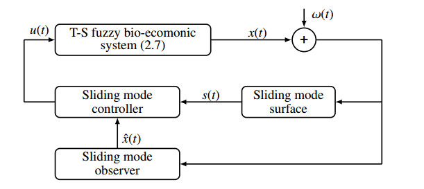
A schematic diagram of the T-S fuzzy bio-economic systems is shown in Figure 1.

3.   Main results

3.1.   Sliding mode observer design

In this paper, we mainly study the population density of alien species. However, in practice, due to various factors and the rapid reproduction of alien species, it is difficult to measure the real population density. Therefore, the design of the state observer usually provides an approximate estimate for the original system. However, it can be observed that since the sliding mode observer has a discontinuous control law, it can deal with the case where the population density is externally excited. Therefore, the observer (3.1) is proposed in this paper.

The functions are as follows:

where $\hat{x}(t) \in {R^n}$ represents the state estimation of $x(t)$, $\hat{y} (t)$ represents the output vector of the observer, ${U_s}\left(t \right)$ represents the input vector of observer and $G$ represents the observer gain to be designed in the sequel.

Define $e(t) = x(t)-\hat{x}(t)$, which represents state estimation error. Subtracting system (3.1) from system (2.7), according to the systems (2.7) and (3.1), we can obtain (3.2) as follows:

3.2.   Construction of sliding surfaces

We first construct the sliding surface for the error system (3.2). The sliding surface is obtained by making $s\left(t \right) = 0$, where the sliding variable $s\left(t \right)$ is defined as

where $S \in {R^{n \times n}}$ is a known matrix satisfying $\det \left({S\bar B} \right) \ne 0$ and $rank\left[{\begin{array}{*{20}{c}}{SE}\\C \end{array}} \right] = rankC$ and $G$ is the observer gain. $Q$ is a known positive definite matrix used to adjust the convergence rate and eliminate the constraint $S\bar J = 0$.

Remark 2. We limit $rank\left[{\begin{array}{*{20}{c}} {SE}\\ C \end{array}} \right] = rank C$, so that there is a matrix $H$ satisfying $SE = HC$, so the sliding variable $s\left(t \right)$ can be converted into

which is accessible.

Compared with the sliding variable without self feedback term, the advantages of the sliding variable (3.6) are mainly reflected in two points: First, the self-feedback term $- Qs\left(t \right)$ allows an increase in the stability margin and makes the sliding variable more robust to disturbances beyond the sliding surface. Second, the self-feedback term is also responsible for eliminating the restrictive constraint $SJ = 0$, stabilizing the sliding variable and reducing chattering. From (3.2) and (3.3), it follows that

When the system is constrained on the sliding surface, we can get $E\left\{ s\left(t \right) \right\} = 0$, so from (3.4), we get $Ls\left(t \right) = 0$. The equivalent control law can be given by ${U_{seq}}\left(t \right) = - {\left({S\bar B} \right)^{ - 1}}S\bar Ae\left(t \right)$. Substituting ${U_{seq}}\left(t \right)$ into (3.2), the sliding mode dynamic can be obtained as

where $\tilde A = \left({I - \bar B{{\left({S\bar B} \right)}^{ - 1}}S} \right)\bar A$.

According to (3.4), the dynamics of sliding variable $s\left(t \right)$ includes a product term $- Qs\left(t \right)$, which involves a Hurwitz matrix $- Q$ and sliding variable itself, which means that the term $- Qs\left(t \right)$ contained in the sliding variable (3.3) has a stabilizing effect on the sliding variable. It can be seen that by introducing $- Qs\left(t \right)$ into the sliding variable $s\left(t \right)$ and selecting an appropriate positive definite matrix $Q$, the convergence speed of the sliding variable can be improved to a certain extent.

By using the state variables of the designed observer, the stability of the system is achieved, and the expected performance is achieved. Therefore, ${s_0} = 0$ can be used to design the observer for (3.1), where

and $K$ is the parameter matrix, so that ${E, \bar A + \bar B}$ are admissible and ${S_0} = {\bar B^T}X \in {R^{m \times n}}$ is the unknown matrix to be determined later.

From (3.4) and (3.6), it follows that

The equivalent control law can be obtained

Further, substituting the equivalent control law into the observer (3.1), we can get the following equation

3.3.   Stability of sliding motion

The dynamics of the resultant sliding motion are given

In order to analyze the mean-square exponentially admissibility of (3.5) and (3.8) simultaneously, the SMO system (3.1) can track the original system (2.7) and the estimation state variables can converge to zero. Thus, we consider the following augmented system:

where

Theorem 3.1. The closed-loop system (3.9) is mean-square exponentially admissible if there are matrices $K, G, X$ and $Y$, and a positive scalar $\alpha$ such that the following inequalities hold:

where

Proof. First, we prove that system (3.9) is impulse free, regular and has a unique solution.

Let

Using (3.10)–(3.12) and (3.16), we have the following equation

Singular invertible matrix results in

Calculated by (3.10) and (3.18),

where ${\Lambda _i}$ and ${\Phi _i}$ are defined in (3.14) and (3.15). It can be seen from Eq (3.16) that the matrix (3.19) is negative definite; that is,

There are non-singular matrixs $M$ and $N$ such that

From (3.17), we can get ${N^T}{\hat E^T}{M^T}{M^{ - T}}\hat ZN = {N^T}{\hat Z^T}{M^{ - 1}}M\hat EN \ge 0$; that is,

By (3.22), we get

then

It follows that (3.20) implies

Moreover, pre-multiplying and post-multiplying Eq (3.25) by ${N^T}$ and $N$ gives us

Since ${\Delta _1}$ and ${\Delta _2}$ are independent of the results discussed below, the actual expressions for these two variables are omitted. From (3.26), we have ${\hat A_{22}}^T{\hat Z_{22}} + {\hat Z_{22}}^T{\hat A_{22}} < 0$, which makes it easy to find ${\hat A_{22}}$ as nonsingular. Therefore, from Eq (3.10), we can obtain the constrained equivalent transformation form of (3.9).

We get system (3.9) as regular and impulse-free. Based on the stochastic theory, the system (3.9) has a unique solution.

Next, we will prove that the system (3.9) is the mean-square exponential stability. Select the Lyapunov function candidate as $V\left({{x_e}\left(t \right), t} \right) = {x_e}^T\left(t \right){\hat E^T}\hat Z{x_e}\left(t \right)$.

Let $W\left(t \right) = {e^{\varepsilon t}}V\left({{x_e}\left(t \right), t} \right)$ and using (3.1), we can obtain

Integrating both sides and then taking expectation yields

By (2.3), we make

which means that

On the basis of (3.31), one can obtain

In terms of ${\hat x_2}\left(t \right) = - {\hat A_{22}}^{ - 1}{\hat A_{21}}{\hat x_1}\left(t \right)$ given by (3.27), one can find positive scalars ${f_1}$ and ${f_2}$ such that

It is noted that

By (3.34) and (3.35), we have

which indicates

From (3.2) and (3.20), we can find a positive scalar $\eta$ so that

Substituting (3.37) into (3.38) and then taking expectation, one has

where $\phi = \dfrac{{\eta ({{f_1} + 1})}}{{{\lambda _{\max }}({{N^{ - T}}{N^{ - 1}}})}}$. Substituting (3.32), (3.33) and (3.39) into (3.29), one has

If $\varepsilon$ is chosen as $\varepsilon \le \frac{\phi }{{{\lambda _{\max }}\left({{{\hat Z}_{11}}} \right)}}$, (3.40) becomes

which indicates

where $\kappa = \frac{E\left(W\left({{t}_{0}} \right) \right)}{{{\lambda }_{\min }}\left({{{\hat{Z}}}_{11}} \right)}$. Using (3.34) and (3.42), one has

It can be seen that system (3.9) is mean-square exponentially admissible.

□

3.4.   Design of sliding mode controllers

Theorem 3.2. Select the appropriate matrix $Q > 0$, $K$ and sliding mode controller

where $\rho = \theta \left\| {S\bar A} \right\| + \partial$. If (3.13) is feasible, then for all $\left\| {x\left(t \right)} \right\| \le \theta$, the sliding mode controller ${U_s}\left(t \right)$ given as above will guarantee that state trajectories of error system (3.2) are attracted to a small ball region around the sliding surface $s\left(t \right) = 0$ from the beginning almost surely.

Proof. We can get

Select the Lyapunov function as $V\left({s\left(t \right)} \right) = \frac{1}{2}{s^T}(t)s(t)$. According to the formula of ${\rm{It\hat o}}$, it is as follows:

where

The reachability condition $LV\left({s\left(t \right)} \right) \le {\alpha _1}\left\| {s\left(t \right)} \right\|$ is satisfied if the following holds

where $\rho \ge {\alpha _1} + \theta \left\| {S\bar A} \right\|$. It can be concluded that the solution of parabolic Eq (3.48) can be divided into two cases: One is that there is a unique solution $\left\| {s\left(t \right)} \right\| = 0$, and the other is that there are two different solutions

where $\Xi = \frac{\sqrt{{{({{\alpha }_{1}}-\partial)}^{2}}+2{{\lambda }_{\min }}(Q){{\lambda }_{\max }}({{J}^{T}}{{S}^{T}}SJ){{\left\| x(t) \right\|}^{2}}}}{2{{\lambda }_{\min }}(Q)}$, $\left\| {s\left(t \right)} \right\| = 0$ can be regarded as a special case of different solutions. Therefore, we only need to analyze the case of two different solutions. According to the parabolic equation in geometry, as long as $\left\| {s\left(t \right)} \right\| \ge {\left\| {s\left(t \right)} \right\|_2}$ is met, (3.48) is true and $\left\| {s\left(t \right)} \right\| \le {\left\| {s\left(t \right)} \right\|_1}$ is discarded due to $\left\| {s\left(t \right)} \right\| \ge 0$ and ${\left\| {s\left(t \right)} \right\|_1} \le 0$.Thus, can get

This means that the sliding variable $s\left(t \right)$ is limited to a ball region

for the beginning almost surely. As a result, the almost sure attractiveness of ball region $\Upsilon \left({s\left(t \right), Q} \right)$ is proved. □

Theorem 3.3. Select the appropriate matrix $Q > 0$, $K$ and sliding mode controller

where $\xi = \rho \left\| {{{({S\bar B})}^{ - 1}}} \right\|\left\| {{S_0}\bar B} \right\| + \mu$ and $\rho = \theta \left\| {S\bar A} \right\| + \partial$. If (3.12) is feasible, for all $\left\| {x\left(t \right)} \right\| \le \theta$, the sliding mode controller $U\left(t \right)$ given above will ensure that the state track of the observer system (3.1) is almost certainly pulled to the sliding surface ${s_0}\left(t \right) = 0$ from the beginning.

Proof. We can get

Select the Lyapunov function as $V\left({{s_0}\left(t \right)} \right) = \frac{1}{2}{s_0}^T\left(t \right){s_0}\left(t \right)$. According to the formula of ${\rm{It\hat o}}$, we have

where

It can be concluded that the sliding variable ${s_0}\left(t \right)$ has been almost always on the sliding surface ${s_0}\left(t \right) = 0$ since the beginning. □

Remark 3. In this paper, we add the product term $- Qs\left(t \right)$ to the sliding variable $s\left(t \right)$ in (3.3) to counteract the $\frac{1}{2}{x^T}\left(t \right){J^T}{S^T}SJx\left(t \right)$ caused by the presence of random noise. Therefore, it is no longer necessary to consider limiting $SJ = 0$. In addition, when $SJ = 0$ is met, the ideal sliding mode appears, and the ball area $Y\left(s\left(t \right), Q \right)$ becomes the sliding surface $s\left(t \right)$ itself. If this happens, the additional robustness of the self feedback item $- Qs\left(t \right)$ will also make the proposed integral sliding variable $s\left(t \right)$ better than the existing sliding variable.

4.   Simulation

Human activities have led to the destruction of the ecological environment of a large number of biological species. For instance, the ocean has been affected by land erosion, which has destroyed the spawning grounds and living environment of young fish. Environmental pollution has also had an increasingly serious impact on people's production and daily life. It is urgent to control and deal with the invasion of alien species.

In the economic globalization today, invasive species has increasingly become a global hot issue. Since the 1980s, alien species have shown a faster growth trend in China. Up to now, nearly 50 new invasive species have been added, and more than 20 dangerous invasive species have successively erupted in large areas in China.

We choose the following parameters according to the case of Nile tilapia:

We have:

where

then ${z_1}\left(t \right)$, ${z_2}\left(t \right)$, ${z_3}\left(t \right)$, ${z_4}\left(t \right)$ and ${z_5}\left(t \right)$ are obtained as follows:

According to the above fuzzy rules given, the fuzzy model is carried out as (2.6). For the expression of ${{A}_{1}}$, ${{A}_{2}}$, ...${{A}_{32}}$, see the appendix. The other expression is as follows:

Set the initial conditions of system (2.6) and observer system to $x(0) = {\left[{\begin{array}{*{20}{c}} { - 7.9} & 3 & {0.8} & { -7.8} & { - 4.9} \end{array}} \right]^T}$ and $\hat x(0) = {\left[{\begin{array}{*{20}{c}} { - 7.9} & 3 & {0.8} & { -7.8} & { - 4.9} \end{array}} \right]^T}$.

The state trajectory of the open loop system (2.6) can be clearly seen in Figure 2, which is not mean-square exponentially admissible. Next, in order to stabilize the system (2.6), a sliding mode control strategy is designed.

It can be obtained that

To design sliding mode control (SMC) laws ${U_s}\left(t \right)$ and $U\left(t \right)$, take appropriate matrices

and $\theta {\rm{ = }}1.5, \partial = 0.001, \mu = 0.001$. Figure 3 shows the trajectory of the closed-loop system, from which it can be found that the state variable of the closed-loop system can converge to zero in a very short time, that is, the observer is asymptotically stable. Figure 4 show the sliding mode surface, respectively. Therefore, the proposed observer and control scheme are effective. To reduce the chattering, by replacing $\dfrac{{s\left(t \right)}}{{\left\| {s\left(t \right)} \right\|}}$ and $\dfrac{{{s_0}\left(t \right)}}{{\left\| {{s_0}\left(t \right)} \right\|}}$ by $\dfrac{{s\left(t \right)}}{{\left\| {s\left(t \right)} \right\| + 0.01}}$ and $\dfrac{{{s_0}\left(t \right)}}{{\left\| {{s_0}\left(t \right)} \right\| + 0.01}}$, as can be seen from Figures 3–6, the simulation results have less chattering and faster convergence. It can be seen that the method of introducing self feedback $- Qs\left(t \right)$ is improved compared with the existing method, which shows that the self feedback item can play a stable role. Therefore, it should be weighed when selecting $Q$.

5.   Conclusions

In this paper, observer-based integral sliding mode control for singular bio-economic system with stochastic fluctuations is studied. A sliding mode observer is designed and an observer based integral sliding mode control method is proposed. By introducing a term consisting of a sliding variable and a negative definite matrix, a new integral sliding surface is constructed. From the results, it can be concluded that the newly introduced term can eliminate restrictive assumptions and has a stabilizing effect on sliding variables. Finally, an example is given to illustrate the effectiveness of the results obtained.

In biology, up to now, we still need to invest in a lot of manpower and material resources to control the density of alien species. The observer-based integral sliding mode control method proposed by us can effectively control the population density of alien invasive species to ensure that native species and invasive species can coexist within a certain range.

Use of AI tools declaration

The authors declare they have not used Artificial Intelligence (AI) tools in the creation of this article.

Conflict of interest

The authors declare there is no conflict of interest in this paper.

Appendix