Time-dependent fractional second-grade fluid flow through a channel influenced by unsteady motion of a bottom plate

Zehba Raizah; Arshad Khan; Saadat Hussain Awan; Anwar Saeed; Ahmed M. Galal; Wajaree Weera; Zehba Raizah; Arshad Khan; Saadat Hussain Awan; Anwar Saeed; Ahmed M. Galal; Wajaree Weera

doi:10.3934/math.2023020

AIMS Mathematics

2023, Volume 8, Issue 1: 423-446. doi: 10.3934/math.2023020

Previous Article Next Article

Research article

Time-dependent fractional second-grade fluid flow through a channel influenced by unsteady motion of a bottom plate

1.
Department of Mathematics, College of Science, Abha, King Khalid University, Saudi Arabia
2.
College of Aeronautical Engineering, National University of Sciences and Technology (NUST), Sector H-12, Islamabad 44000, Pakistan
3.
Department of Mathematics, Abdul Wali Khan University, Mardan, 23200, Khyber, Pakhtunkhwa, Pakistan
4.
Department of Mechanical Engineering, College of Engineering in Wadi Alddawasir, Prince Sattam bin Abdulaziz University, Saudi Arabia
5.
Production Engineering and Mechanical Design Department, Faculty of Engineering, Mansoura University, P.O 35516, Mansoura, Egypt
6.
Department of Mathematics, Faculty of Science, Khon Kaen University, Khon Kaen, 40002, Thailand

Received: 29 June 2022 Revised: 06 September 2022 Accepted: 20 September 2022 Published: 08 October 2022
MSC : 26A33, 42A38, 44A10, 44A35

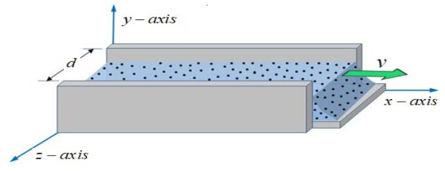
This investigation theoretically describes the exact solution of an unsteady fractional a second-grade fluid upon a bottom plate constrained by two walls at the sides which are parallel to each other and are normal to the bottom plate. The flow in the fluid is induced by the time dependent motion of the bottom plate. Initially the flow equation along with boundary and initial conditions are considered which are then transformed to dimensionless notations using suitable set of variables. The Laplace as well as Fourier transformations have been employed to recover the exact solution of flow equation. The time fractional differential operator of Caputo-Fabrizio has been employed to have constitutive equations of fractional order for second-grade fluid. After obtaining the general exact solutions for flow characteristics, three different cases at the surface of bottom plate are discussed; namely (i) Stokes first problem (ii) Accelerating flow (iii) Stokes second problem. It has noticed in this study that, for higher values of Reynolds number the flow characteristics have augmented in all the three cases. Moreover, higher values of time variable have supported the flow of fractional fluid for impulsive and constantly accelerated motion and have opposeed the flow for sine and cosine oscillations.
- Caputo-Fabrizio Operator,
- Non-Newtonian fluid,
- Channel flow,
- unsteady flow,
- Laplace transform,
- Fourier transform,
- second grade fluid
Citation: Zehba Raizah, Arshad Khan, Saadat Hussain Awan, Anwar Saeed, Ahmed M. Galal, Wajaree Weera. Time-dependent fractional second-grade fluid flow through a channel influenced by unsteady motion of a bottom plate[J]. AIMS Mathematics, 2023, 8(1): 423-446. doi: 10.3934/math.2023020

Related Papers:

Abstract

This investigation theoretically describes the exact solution of an unsteady fractional a second-grade fluid upon a bottom plate constrained by two walls at the sides which are parallel to each other and are normal to the bottom plate. The flow in the fluid is induced by the time dependent motion of the bottom plate. Initially the flow equation along with boundary and initial conditions are considered which are then transformed to dimensionless notations using suitable set of variables. The Laplace as well as Fourier transformations have been employed to recover the exact solution of flow equation. The time fractional differential operator of Caputo-Fabrizio has been employed to have constitutive equations of fractional order for second-grade fluid. After obtaining the general exact solutions for flow characteristics, three different cases at the surface of bottom plate are discussed; namely (i) Stokes first problem (ii) Accelerating flow (iii) Stokes second problem. It has noticed in this study that, for higher values of Reynolds number the flow characteristics have augmented in all the three cases. Moreover, higher values of time variable have supported the flow of fractional fluid for impulsive and constantly accelerated motion and have opposeed the flow for sine and cosine oscillations.

References

[1]	M. Caputo, M. Fabrizio, A new definition of fractional derivative without singular kernel, Progr. Fract. Differ. Appl., 1 (2015), 1–13. http://doi.org/10.12785/pfda/010201 doi: 10.12785/pfda/010201
[2]	A. Alshabanat, M. Jleli, S. Kumar, B. Samet, Generalization of Caputo-Fabrizio fractional derivative and applications to electrical circuits, Front. Phys., 8 (2020), 1–10. https://doi.org/10.3389/fphy.2020.00064 doi: 10.3389/fphy.2020.00064
[3]	M. Hamid, T. Zubair, M. Usman, R. U. Haq, Numerical investigation of fractional-order unsteady natural convective radiating flow of nanofluid in a vertical channel, AIMS Math., 4 (2019), 1416–1429. http://doi:10.3934/math.2019.5.1416 doi: 10.3934/math.2019.5.1416
[4]	J. Singh, D. Kumar, Z. Hammouch, A. Atangana, A fractional epidemiological model for computer viruses pertaining to a new fractional derivative, Appl. Math. Comput., 316 (2018), 504–515. https://doi.org/10.1016/j.amc.2017.08.048 doi: 10.1016/j.amc.2017.08.048
[5]	N. A. Shah, I. Khan, Heat transfer analysis in a second grade fluid over and oscillating vertical plate using fractional Caputo-Fabrizio derivatives. Eur. Phys. J. C, 76 (2016), 1–11. https://doi.org/10.1140/epjc/s10052-016-4209-3 doi: 10.1140/epjc/s10052-016-4209-3
[6]	M. Hamid, M. Usman, Y. Yan, Z. Tian, An efficient numerical scheme for fractional characterization of MHD fluid model, Chaos Soliton. Fract., 162 (2022), 1–13. https://doi.org/10.1016/j.chaos.2022.112475 doi: 10.1016/j.chaos.2022.112475
[7]	M. Usman, W. Alhejaili, M. Hamid, N. Khan, Fractional analysis of Jeffrey fluid over a vertical plate with time-dependent conductivity and diffusivity: A low-cost spectral approach, J. Comput. Sci., 63 (2022), 101769. https://doi.org/10.1016/j.jocs.2022.101769 doi: 10.1016/j.jocs.2022.101769
[8]	M. Hamid, M. Usman, W. Wang, Z. Tian, Hybrid fully spectral linearized scheme for time‐fractional evolutionary equations, Math. Methods Appl. Sci., 44 (2021), 3890–3912. https://doi.org/10.1002/mma.6996 doi: 10.1002/mma.6996
[9]	M. Hamid, M. Usman, R. U. Haq, W. Wang, A Chelyshkov polynomial based algorithm to analyze the transport dynamics and anomalous diffusion in fractional model, Phys. A: Stat. Mech. Appl., 551 (2020), 124227. https://doi.org/10.1016/j.physa.2020.124227 doi: 10.1016/j.physa.2020.124227
[10]	M. Hamid, M. Usman, W. Wang, Z. Tian, A stable computational approach to analyze semi‐relativistic behavior of fractional evolutionary problems, Numer. Methods Partial Differ. Equ., 38 (2022), 122–136. https://doi.org/10.1002/num.22617 doi: 10.1002/num.22617
[11]	F. Ali, I. Khan, S. Shafie, Closed form solutions for unsteady free convection flow of a second grade fluid over an oscillating vertical plate, PLoS One, 9 (2014), e85099. https://doi.org/10.1371/journal.pone.0085099 doi: 10.1371/journal.pone.0085099
[12]	A. Taha, A. Aziz, C. M. Khalique, Exact solutions for Stokes' Flow of a Non-Newtonian nanofluid model: A Lie similarity approach, Z. Naturforsch. A, 71 (2016), 621–630. https://doi.org/10.1515/zna-2016-0031 doi: 10.1515/zna-2016-0031
[13]	C. J. Toki, J. N. Tokis, Exact solutions for the unsteady free convection flows on a porous plate with time-dependent heating, ZAMM-Z. Angew. Math. Me., 87 (2007), 4–13. https://doi.org/10.1002/zamm.200510291 doi: 10.1002/zamm.200510291
[14]	M. Asif, S. U. Haq, S. Islam, I. Khan, I. Tlili, Exact solution of non-Newtonian fluid motion between side walls, Results Phys., 11 (2018), 534–539. https://doi.org/10.1016/j.rinp.2018.09.023 doi: 10.1016/j.rinp.2018.09.023
[15]	B. K. Jha, A. O. Ajibade, Free convection heat and mass transfer flow in a vertical channel with the Dufour effect, J. Mech. Eng., 224 (2010), 91–101. https://doi.org/10.1243/09544089JPME318 doi: 10.1243/09544089JPME318
[16]	D. B. Ingham, Transient free convection on an isothermal vertical flat plate, Int. J. Heat Mass Trans., 21 (1978), 67–69. https://doi.org/10.1016/0017-9310(78)90159-X doi: 10.1016/0017-9310(78)90159-X
[17]	A. Raptis, A. K. Singh, MHD free convection flow past an accelerated vertical plate, Int. Commun. Heat Mass Transf., 10 (1983), 313–321. https://doi.org/10.1016/0735-1933(83)90016-7 doi: 10.1016/0735-1933(83)90016-7
[18]	A. K. Singh, N. Kumar, Free-convection flow past an exponentially accelerated vertical plate, Astrophys. Space Sci., 98 (1984), 245–248. https://doi.org/10.1007/BF00651403 doi: 10.1007/BF00651403
[19]	M. Khan, R. Malik, A. Anjum, Analytic solutions for MHD flow of an Oldroyd-B fluid between two side walls perpendicular to the plate, Chem. Eng. Commun., 198 (2011), 1415–1434. https://doi.org/10.1080/00986445.2011.560521 doi: 10.1080/00986445.2011.560521
[20]	S. U. Haq, A. ur Rahman, I. Khan, F. Ali, S. I. A. Shah, The impact of side walls on the MHD flow of a second-grade fluid through a porous medium, Neural. Comput. Appl., 30 (2016), 1103–1109. https://doi.org/10.1007/s00521-016-2733-6 doi: 10.1007/s00521-016-2733-6
[21]	C. Fetecau, Analytical solutions for non-Newtonian fluid flows in pipe-like domains, Int. J. Nonliner Mech., 39 (2004), 225–231. https://doi.org/10.1016/S0020-7462(02)00170-1 doi: 10.1016/S0020-7462(02)00170-1
[22]	R. Bandelli, K. R. Rajagopal, Start-up flows of second grade fluids in domains with one finite dimension, Int. J. Nonliner Mech., 30 (1995), 817–839. https://doi.org/10.1016/0020-7462(95)00035-6 doi: 10.1016/0020-7462(95)00035-6
[23]	C. Fetecau, T. Hayat, C. Fetecau, N. Ali, Unsteady flow of a second grade fluid between two side walls perpendicular to a plate, Nonlinear Anal. Real World Appl., 9 (2008), 1236–1252. https://doi.org/10.1016/j.nonrwa.2007.02.014 doi: 10.1016/j.nonrwa.2007.02.014
[24]	C. Fetecǎu, J. Zierep, On a class of exact solutions of the equations of motion of a second grade fluid, Acta Mech., 150 (2001), 135–138. https://doi.org/10.1007/BF01178551 doi: 10.1007/BF01178551
[25]	I. S. Gradshteyn, I. M. Ryzhik, Table of Integrals, Series, and Products Seventh Edition, Academic Press (Elsevier): Burlington, MA and London, UK, (2007). https://doi.org/10.1016/C2009-0-22516-5
[26]	L. Debnath, D. Bhatta, Integral Transforms and Their Applications Second Edition, Chapman & Hall/CRC Taylor & Francis Group, 2006. https://doi.org/10.1201/9781420010916 doi: 10.1201/9781420010916
[27]	S. U. Haq, M. A. Khan, Z. A. Khan, F. Ali, MHD effects on the channel flow of a fractional viscous fluid through a porous medium: An application of the Caputo-Fabrizio time-fractional derivative, Chin. J. Phys., 65 (2020), 14–23. https://doi.org/10.1016/j.cjph.2020.02.014 doi: 10.1016/j.cjph.2020.02.014

Reader Comments

Your name:*

Email:*
© 2023 the Author(s), licensee AIMS Press. This is an open access article distributed under the terms of the Creative Commons Attribution License (http://creativecommons.org/licenses/by/4.0)