Dynamic analysis of fractional-order neural networks with inertia

Zhiying Li; Wangdong Jiang; Yuehong Zhang; Zhiying Li; Wangdong Jiang; Yuehong Zhang

doi:10.3934/math.2022927

AIMS Mathematics

2022, Volume 7, Issue 9: 16889-16906. doi: 10.3934/math.2022927

Previous Article Next Article

Research article

Dynamic analysis of fractional-order neural networks with inertia

The Fundamental Education Department of Yuanpei College, Shaoxing University, Shaoxing 312000, China

Received: 23 May 2022 Revised: 28 June 2022 Accepted: 01 July 2022 Published: 15 July 2022
MSC : 45M05

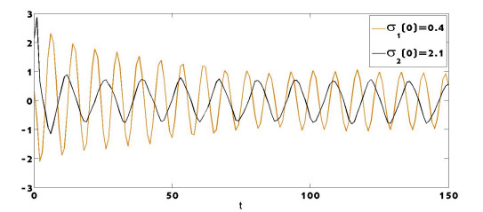
The existence and the S-asymptotic $ \omega $-periodic of the solution in fractional-order Cohen-Grossberg neural networks with inertia are studied in this paper. Based on the properties of the Riemann-Liouville (R-L) fractional-order derivative and integral, the contraction mapping principle, and the Arzela-Ascoli theorem, sufficient conditions for the existence and the S-asymptotic $ \omega $-period of the system are achieved. In addition, an example is simulated to testify the theorem.
- fractional-order neural networks,
- contraction mapping principle,
- inertia,
- existence,
- S-asymptotic $ \omega $-periodic
Citation: Zhiying Li, Wangdong Jiang, Yuehong Zhang. Dynamic analysis of fractional-order neural networks with inertia[J]. AIMS Mathematics, 2022, 7(9): 16889-16906. doi: 10.3934/math.2022927

Related Papers:

Abstract

The existence and the S-asymptotic $ \omega $-periodic of the solution in fractional-order Cohen-Grossberg neural networks with inertia are studied in this paper. Based on the properties of the Riemann-Liouville (R-L) fractional-order derivative and integral, the contraction mapping principle, and the Arzela-Ascoli theorem, sufficient conditions for the existence and the S-asymptotic $ \omega $-period of the system are achieved. In addition, an example is simulated to testify the theorem.

References

[1]	V. Lakshmikantham, S. Leela, J. V. Devi, Theory of fractional dynamic systems, Cambridge Scientific Publishers Ltd., 2009.
[2]	C. P. Li, W. H. Deng, Remarks on fractional derivatives, Appl. Math. Comput, 187 (2007), 777–784. https://doi.org/10.1016/j.amc.2006.08.163 doi: 10.1016/j.amc.2006.08.163
[3]	A. Kilbas, H. M. SrivastavaH, J. J. Trujillo, Theory and applications of fractional differential equations, Amsterdan: Elsevier, 2006.
[4]	I. Podlubny, Franctional differential equations, New York: Academic Press, 1999.
[5]	O. Heaviside, Electromagnetic theory, New York: Chelsea, 1971.
[6]	H. Sun, A. Abdelwahab, B. Onaral, Linear approximation of transfer function with a pole of fractional power, IEEE T. Automat. Contr., 29 (1984), 441–444. https://doi.org/10.1109/TAC.1984.1103551 doi: 10.1109/TAC.1984.1103551
[7]	R. C. Koeller, Application of fractional calculus to the theory of viscoelasticity, J. Appl. Mech., 51 (1984), 299–307. https://doi.org/10.1115/1.3167616 doi: 10.1115/1.3167616
[8]	W. C. Chen, Nonlinear dynamics and chaos in a fractional-order finacial system, Chaos Solition. Fract., 36 (2008), 1305–1314. https://doi.org/10.1016/j.chaos.2006.07.051 doi: 10.1016/j.chaos.2006.07.051
[9]	T. J. Anastasio, The fractional-order dynamics of brainstem vestibulo-oculomotor neurons, Biolo. Cybern., 72 (1994), 69–79. https://doi.org/10.1007/BF00206239 doi: 10.1007/BF00206239
[10]	C. J. Xu, P. L. Li, On finite-time Stability for fractional-order neural networks with proportional delays, Neural Process. Lett., 50 (2019), 1241–1256. https://doi.org/10.1007/s11063-018-9917-2 doi: 10.1007/s11063-018-9917-2
[11]	J. D. Li, Z. B. Wu, N. J. Huang, Asymptotical stability of Riemann-Liouville fractional neutral-type delayed projective neural networks, Neural Process. Lett., 50 (2019), 565–579. https://doi.org/10.1007/s11063-019-10050-8 doi: 10.1007/s11063-019-10050-8
[12]	F. Y. Zhou, C. Y. Ma, Mittag-Leffler stability and global asymptotically $\omega-$periodicity of fractional BAM neural networks with time-varying delays, Neural Process. Lett., 47 (2018), 71–98. https://doi.org/10.1007/s11063-017-9634-2 doi: 10.1007/s11063-017-9634-2
[13]	C. J. Xu, W. Zhang, C. Aouiti, Z. X. Liu, M. X. Liao, P. L. Li, Further investigation on bifurcation and their control of fractional-order BAM neural networks involving four neurons and multiple delays, Math. Method. Appl. Sci., 2021. https://doi.org/10.1002/mma.7581 doi: 10.1002/mma.7581
[14]	S. C. Xu, X. Y. Wang, X. L. Ye, A new fractional-order chaos system of Hopfield neural network and its application in image encryption, Chaos Soliton. Fract., 157 (2022), 111889. https://doi.org/10.1016/j.chaos.2022.111889 doi: 10.1016/j.chaos.2022.111889
[15]	Y. R. Liu, L. Wang, K. X. Gu, M. Li, Artificial Neural Network (ANN)–Bayesian probability framework (BPF) based method of dynamic force reconstruction under multi-source uncertainties, Knowl.-Based Syst., 237 (2022), 107796. https://doi.org/10.1016/j.knosys.2021.107796 doi: 10.1016/j.knosys.2021.107796
[16]	A. Mauro, F. Conti, F. Dodge, R. Schor, Subthreshold behavior and phenomenological impedance of the squid giant axon, J. Gen. Physiol., 55 (1970), 497–523. https://doi.org/10.1085/jgp.55.4.497 doi: 10.1085/jgp.55.4.497
[17]	D. E. Angelaki, M. J. Correia, Models of membrane resonance in pigeon semicircular canal type Ⅱ hair cells, Biol. Cybern., 65 (1991), 1–10. https://doi.org/10.1007/BF00197284 doi: 10.1007/BF00197284
[18]	J. F. Ashmore, D. Attwell, Models for electrical tuning in hair cells, Proc. Royal Soc. B: Biol. Sci., 226 (1985), 325–344.
[19]	L. Ke, W. L. Li, Exponential synchronization in inertial Cohen-Grossberg neural networks with time delays, J. Franklin I., 356 (2019), 11285–11304. https://doi.org/10.1016/j.jfranklin.2019.07.027 doi: 10.1016/j.jfranklin.2019.07.027
[20]	L. Ke, W. L. Li, Exponential synchronization in inertial neural networks with time delays, Electronics, 8 (2019), 356. https://doi.org/10.3390/electronics8030356 doi: 10.3390/electronics8030356
[21]	S. Li, X. M. Wang, H. Y. Qin, X. M. Zhong, Synchronization criteria for neutral-type quaternion-valued neural networks with mixed delays, AIMS Mathematics, 6 (2021), 8044–8063. https://doi.org/10.3934/math.2021467 doi: 10.3934/math.2021467
[22]	F. C. Kong, Q. X. Zhu, R. Sakthivel, A. Mohammadzadeh, Fixed-time synchronization analysis for discontinuous fuzzy inertial neural networks with parameter uncertainties, Neurocomputing, 422 (2021), 295–313. https://doi.org/10.1016/j.neucom.2020.09.014 doi: 10.1016/j.neucom.2020.09.014
[23]	W. Zhang, J. T. Qi, Synchronization of coupled memristive inertial delayed neural networks with impulse and intermittent control, Neural Comput. Appl., 33 (2020), 7953–7964. https://doi.org/10.1007/s00521-020-05540-z doi: 10.1007/s00521-020-05540-z
[24]	L. Ke, Mittag-Leffler stability and asymptotic $\omega$-periodicity of fractional inertial neural networks with time-delays, Neurocomputing, 465 (2021), 53–62. https://doi.org/10.1016/j.neucom.2021.08.121 doi: 10.1016/j.neucom.2021.08.121
[25]	H. R. Henriquez, M. Pjerri, P. Tboas, On S-asymptotically $\omega$-periodicityic functions on Banach spaces and applications, J. Math. Anal. Appl., 343 (2008), 1119–1130. https://doi.org/10.1016/j.jmaa.2008.02.023 doi: 10.1016/j.jmaa.2008.02.023
[26]	Y. J. Gu, H. Wang, Y. G. Yu, Stability and synchronization for Riemann-Liouville fractional time-delayed inertial neural networks, Neurocomputing, 340 (2019), 270–280. https://doi.org/10.1016/j.neucom.2019.03.005 doi: 10.1016/j.neucom.2019.03.005
[27]	S. L. Zhang, M. L. Tang, X. G. Liu, Synchronization of a Riemann-Liouville fractional time-delayed neural network with two inertial terms, Circuits Syst. Signal Process., 40 (2021), 5280–5308. https://doi.org/10.1007/s00034-021-01717-6 doi: 10.1007/s00034-021-01717-6
[28]	M. A. Cohen, S. Grossberg, Absolute stability of global pattern formation and parallel memory storage by competitive neural networks, IEEE T. Syst. Man. Cy., SMC-13 (1983), 815–826. https://doi.org/10.1109/TSMC.1983.6313075 doi: 10.1109/TSMC.1983.6313075
[29]	M. A. Krasnoselskii, Topological methods in the theory of nonlinear integral equations, 1964.

Reader Comments

Your name:*

Email:*
© 2022 the Author(s), licensee AIMS Press. This is an open access article distributed under the terms of the Creative Commons Attribution License (http://creativecommons.org/licenses/by/4.0)