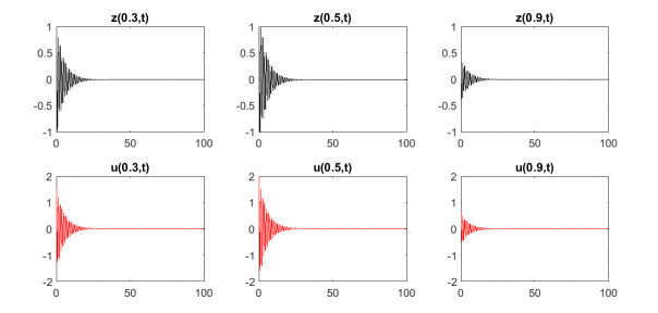
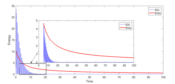
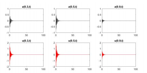
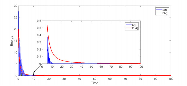
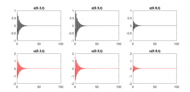
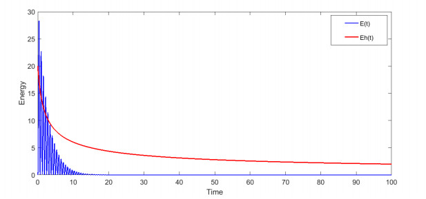
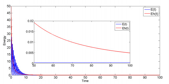
The purpose of this paper is to establish a general stability result for a one-dimensional linear swelling porous-elastic system with past history, irrespective of the wave speeds of the system. First, we establish an explicit and general decay result under a wider class of the relaxation (kernel) functions. The kernel in our memory term is more general and of a broader class. Further, we get a better decay rate without imposing some assumptions on the boundedness of the history data considered in many earlier results in the literature. We also perform several numerical tests to illustrate our theoretical results. Our output extends and improves some of the available results on swelling porous media in the literature.
Citation: Adel M. Al-Mahdi, Mohammad M. Al-Gharabli, Mohamed Alahyane. Theoretical and numerical stability results for a viscoelastic swelling porous-elastic system with past history[J]. AIMS Mathematics, 2021, 6(11): 11921-11949. doi: 10.3934/math.2021692
The purpose of this paper is to establish a general stability result for a one-dimensional linear swelling porous-elastic system with past history, irrespective of the wave speeds of the system. First, we establish an explicit and general decay result under a wider class of the relaxation (kernel) functions. The kernel in our memory term is more general and of a broader class. Further, we get a better decay rate without imposing some assumptions on the boundedness of the history data considered in many earlier results in the literature. We also perform several numerical tests to illustrate our theoretical results. Our output extends and improves some of the available results on swelling porous media in the literature.

| [1] |
M. A. Goodman, S. C. Cowin, A continuum theory for granular materials, Arch. Rational Mech. Anal., 44 (1972), 249–266, doi: 10.1007/BF00284326

|
| [2] |
J. W. Nunziato, S. C. Cowin, A nonlinear theory of elastic materials with voids, Arch. Rational Mech. Anal., 72 (1979), 175–201. doi: 10.1007/BF00249363
|
| [3] |
D. Ieșan, R. Quintanilla, A theory of porous thermoviscoelastic mixtures, J. Therm. Stresses, 30 (2007), 693–714. doi: 10.1080/01495730701212880
|
| [4] |
P. S. Casas, R. Quintanilla, Exponential decay in one-dimensional porous-thermo-elasticity, Mech. Res. Commun., 32 (2005), 652–658. doi: 10.1016/j.mechrescom.2005.02.015
|
| [5] |
P. S. Casas, R. Quintanilla, Exponential stability in thermoelasticity with microtemperatures, Int. J. Eng. Sci., 43 (2005), 33–47. doi: 10.1016/j.ijengsci.2004.09.004
|
| [6] |
A. Magaña, R. Quintanilla, On the time decay of solutions in one-dimensional theories of porous materials, Int. J. Solids Struct., 43 (2006), 3414–3427. doi: 10.1016/j.ijsolstr.2005.06.077
|
| [7] |
P. X. Pamplona, J. E. M. Rivera, R. Quintanilla, Stabilization in elastic solids with voids, J. Math. Anal. Appl., 350 (2009), 37–49. doi: 10.1016/j.jmaa.2008.09.026
|
| [8] |
A. Magaña, R. Quintanilla, On the time decay of solutions in porous-elasticity with quasi-static microvoids, J. Math. Anal. Appl., 331 (2007), 617–630. doi: 10.1016/j.jmaa.2006.08.086
|
| [9] |
J. Muñoz-Rivera, R. Quintanilla, On the time polynomial decay in elastic solids with voids, J. Math. Anal. Appl., 338 (2008), 1296–1309. doi: 10.1016/j.jmaa.2007.06.005
|
| [10] |
A. Soufyane, Energy decay for porous-thermo-elasticity systems of memory type, Appl. Anal., 87 (2008), 451–464. doi: 10.1080/00036810802035634
|
| [11] | A. Soufyane, M. Afilal, M. Chacha, Boundary stabilization of memory type for the porous-thermo-elasticity system, Abstr. Appl. Anal., 2009 (2009), 280790. |
| [12] |
A. Soufyane, M. Afilal, T. Aouam, M. Chacha, General decay of solutions of a linear one-dimensional porous-thermoelasticity system with a boundary control of memory type, Nonlinear Anal.-Theor., 72 (2010), 3903–3910. doi: 10.1016/j.na.2010.01.004
|
| [13] |
P. X. Pamplona, J. E. M. Rivera, R. Quintanilla, On the decay of solutions for porous-elastic systems with history, J. Math. Anal. Appl., 379 (2011), 682–705. doi: 10.1016/j.jmaa.2011.01.045
|
| [14] |
S. A. Messaoudi, A. Fareh, General decay for a porous thermoelastic system with memory: The case of equal speeds, Nonlinear Anal.-Theor., 74 (2011), 6895–6906. doi: 10.1016/j.na.2011.07.012
|
| [15] |
S. A. Messaoudi, A. Fareh, General decay for a porous-thermoelastic system with memory: the case of nonequal speeds, Acta Math. Sci., 33 (2013), 23–40. doi: 10.1016/S0252-9602(12)60192-1
|
| [16] |
S. A. Messaoudi, A. Fareh, Exponential decay for linear damped porous thermoelastic systems with second sound, DCDS-B, 20 (2015), 599–612. doi: 10.3934/dcdsb.2015.20.599
|
| [17] |
Z.-J. Han, G.-Q. Xu, Exponential decay in non-uniform porous-thermo-elasticity model of lord-shulman type, DCDS-B, 17 (2012), 57–77. doi: 10.3934/dcdsb.2012.17.57
|
| [18] |
B. Said-Houari, S. A. Messaoudi, Decay property of regularity-loss type of solutions in elastic solids with voids, Appl. Anal., 92 (2013), 2487–2507. doi: 10.1080/00036811.2012.742188
|
| [19] |
T. A. Apalara, General decay of solutions in one-dimensional porous-elastic system with memory, J. Math. Anal. Appl., 469 (2019), 457–471. doi: 10.1016/j.jmaa.2017.08.007
|
| [20] |
B. W. Feng, M. Y. Yin, Decay of solutions for a one-dimensional porous elasticity system with memory: the case of non-equal wave speeds, Math. Mech. Solids, 24 (2019), 2361–2373. doi: 10.1177/1081286518757299
|
| [21] |
M. L. Santos, A. D. S. Campelo, M. L. S. Oliveira, On porous-elastic systems with fourier law, Appl. Anal., 98 (2019), 1181–1197. doi: 10.1080/00036811.2017.1419197
|
| [22] |
M. L. Santos, A. D. S. Campelo, D. S. A. Júnior, On the decay rates of porous elastic systems, J. Elast., 127 (2017), 79–101. doi: 10.1007/s10659-016-9597-y
|
| [23] |
T. A. Apalara, A general decay for a weakly nonlinearly damped porous system, J. Dyn. Control Syst., 25 (2019), 311–322. doi: 10.1007/s10883-018-9407-x
|
| [24] |
B. W. Feng, T. A. Apalara, Optimal decay for a porous elasticity system with memory, J. Math. Anal. Appl., 470 (2019), 1108–1128. doi: 10.1016/j.jmaa.2018.10.052
|
| [25] | V. Hung, Hidden disaster, University News, University of Saska Techwan, Saskatoon, Canada, 2003. |
| [26] |
M. M. Freitas, A. J. A. Ramos, M. L. Santos, Existence and upper-semicontinuity of global attractors for binary mixtures solids with fractional damping, Appl.Math. Optim, 83 (2021), 1353–1385. doi: 10.1007/s00245-019-09590-1
|
| [27] |
T. K. Karalis, On the elastic deformation of non-saturated swelling soils, Acta Mechanica, 84 (1990), 19–45. doi: 10.1007/BF01176086
|
| [28] | R. L. Handy, A stress path model for collapsible loess, In: Genesis and properties of collapsible soils, Springer, 1995, 33–47, |
| [29] | R. Leonard, Expansive soils, Shallow Foundation, Kansas, USA, Regent Centre, University of Kansas, 1989. |
| [30] | L. D. Jones, I. Jefferson, Expansive soils, In: ICE manual of geotechnical engineering, ICE Publishing, 1 (2012), 413–441. |
| [31] | J. E. Bowles, Foundation design and analysis, New York: McGraw-Hill, Book Co., Inc., 1982. |
| [32] | B. Kalantari, Engineering significant of swelling soils, Res. J. Appl. Sci. Eng. Technol., 4 (2012), 2874–2878. |
| [33] |
D. Ieșan, On the theory of mixtures of thermoelastic solids, J. Therm. Stresses, 14 (1991), 389–408. doi: 10.1080/01495739108927075
|
| [34] |
R. Quintanilla, Exponential stability for one-dimensional problem of swelling porous elastic soils with fluid saturation, J. Comput. Appl. Math., 145 (2002), 525–533. doi: 10.1016/S0377-0427(02)00442-9
|
| [35] |
J. M. Wang, B. Z. Guo, On the stability of swelling porous elastic soils with fluid saturation by one internal damping, IMA J. Appl. Math., 71 (2006), 565–582. doi: 10.1093/imamat/hxl009
|
| [36] |
A. J. A. Ramos, M. M. Freitas, D. S. Almeida Jr, A. S. Noé, M. D. J. Santos, Stability results for elastic porous media swelling with nonlinear damping, J. Math. Phys., 61 (2020), 101505. doi: 10.1063/5.0014121
|
| [37] |
T. A. Apalara, General stability result of swelling porous elastic soils with a viscoelastic damping, Z. Angew. Math. Phys., 71 (2020), 200. doi: 10.1007/s00033-020-01427-0
|
| [38] |
T. A. Apalara, General stability of memory-type thermoelastic timoshenko beam acting on shear force, Continuum Mech. Thermodyn., 30 (2018), 291–300. doi: 10.1007/s00161-017-0601-y
|
| [39] |
F. A.-Khodja, A. Benabdallah, J. E. M. Rivera, R. Racke, Energy decay for timoshenko systems of memory type, J. Differ. Equations, 194 (2003), 82–115. doi: 10.1016/S0022-0396(03)00185-2
|
| [40] |
A. M. Al-Mahdi, M. M. Al-Gharabli, A. Guesmia, S. A. Messaoudi, New decay results for a viscoelastic-type timoshenko system with infinite memory, Z. Angew. Math. Phys., 72 (2021), 22, doi: 10.1007/s00033-020-01446-x
|
| [41] | D. S. A. Júnior, A. J. A. Ramos, A. S. Noé, M. M. Freitas, P. T. Aum, Stabilization and numerical treatment for swelling porous elastic soils with fluid saturation, ZAMM, 2021, DOI: 10.1002/zamm.202000366. |
| [42] |
A. J. A. Ramos, D. S. A. Almeida Júnior, M. M. Freitas, A. S. Noé, M. J. D. Santos, Stabilization of swelling porous elastic soils with fluid saturation and delay time terms, J. Math. Phys., 62 (2021), 021507. doi: 10.1063/5.0018795
|
| [43] |
J. A. D. Appleby, M. Fabrizio, B. Lazzari, D. W. Reynolds, On exponential asymptotic stability in linear viscoelasticity, Math. Mod. Meth. Appl. S., 16 (2006), 1677–1694. doi: 10.1142/S0218202506001674
|
| [44] |
V. Pata, Stability and exponential stability in linear viscoelasticity, Milan J. Math., 77 (2009), 333. doi: 10.1007/s00032-009-0098-3
|
| [45] |
A. Guesmia, S. A. Messaoudi, A general decay result for a viscoelastic equation in the presence of past and finite history memories, Nonlinear Anal.-Real, 13 (2012), 476–485. doi: 10.1016/j.nonrwa.2011.08.004
|
| [46] |
A. Guesmia, Asymptotic stability of abstract dissipative systems with infinite memory, J. Math. Anal. Appl., 382 (2011), 748–760. doi: 10.1016/j.jmaa.2011.04.079
|
| [47] | M. I. Mustafa, Energy decay in a quasilinear system with finite and infinite memories, In: Mathematical methods in egineering, Springer, 2019,235–256, |
| [48] |
A. M. Al-Mahdi, M. M. Al-Gharabli, New general decay results in an infinite memory viscoelastic problem with nonlinear damping, Bound. Value Probl., 2019 (2019), 140. doi: 10.1186/s13661-019-1253-6
|
| [49] | A. Youkana, Stability of an abstract system with infinite history, 2018, arXiv: 1805.07964. |
| [50] |
A. M. Al-Mahdi, General stability result for a viscoelastic plate equation with past history and general kernel, J. Math. Anal. Appl., 490 (2020), 124216. doi: 10.1016/j.jmaa.2020.124216
|
| [51] |
A. M. Al-Mahdi, Stability result of a viscoelastic plate equation with past history and a logarithmic nonlinearity, Bound. Value Probl., 2020 (2020), 84. doi: 10.1186/s13661-020-01382-9
|
| [52] |
A. Guesmia, New general decay rates of solutions for two viscoelastic wave equations with infinite memory, Math. Model. Anal., 25 (2020), 351–373. doi: 10.3846/mma.2020.10458
|
| [53] |
A. Guesmia, Asymptotic stability of abstract dissipative systems with infinite memory, J. Math. Anal. Appl., 382 (2011), 748–760. doi: 10.1016/j.jmaa.2011.04.079
|
| [54] |
A. Guesmia, S. A. Messaoudi, A new approach to the stability of an abstract system in the presence of infinite history, J. Math. Anal. Appl., 416 (2014), 212–228. doi: 10.1016/j.jmaa.2014.02.030
|
| [55] |
M. I. Mustafa, Optimal decay rates for the viscoelastic wave equation, Math. Meth. Appl. Sci., 41 (2018), 192–204. doi: 10.1002/mma.4604
|
| [56] |
M. M. Al-Gharabli, A. M. Al-Mahdi, S. A. Messaoudi, General and optimal decay result for a viscoelastic problem with nonlinear boundary feedback, J. Dyn. Control Syst., 25 (2019), 551–572. doi: 10.1007/s10883-018-9422-y
|
| [57] | V. I. Arnold, Mathematical methods of classical mechanics, Berlin and New York: Springer, 1989. |

Figures(9)

Adel M. Al-Mahdi, Mohammad M. Al-Gharabli, Mohamed Alahyane. Theoretical and numerical stability results for a viscoelastic swelling porous-elastic system with past history[J]. AIMS Mathematics, 2021, 6(11): 11921-11949. doi: 10.3934/math.2021692


 DownLoad: