Stabilization of a viscoelastic wave equation with boundary damping and variable exponents: Theoretical and numerical study

Adel M. Al-Mahdi; Mohammad M. Al-Gharabli; Maher Nour; Mostafa Zahri; Adel M. Al-Mahdi; Mohammad M. Al-Gharabli; Maher Nour; Mostafa Zahri

doi:10.3934/math.2022842

AIMS Mathematics

2022, Volume 7, Issue 8: 15370-15401. doi: 10.3934/math.2022842

Previous Article Next Article

Research article Special Issues

Stabilization of a viscoelastic wave equation with boundary damping and variable exponents: Theoretical and numerical study

1.
The Preparatory Year Program, King Fahd University of Petroleum and Minerals, Dhahran 31261, Saudi Arabia
2.
The Interdisciplinary Research Center in Construction and Building Materials, King Fahd University of Petroleum and Minerals, Dhahran 31261, Saudi Arabia
3.
DCC-Math, King Fahd University of Petroleum and Minerals, Dhahran 31261, Saudi Arabia
4.
Department of Mathematics, College of Sciences, Research Groups MASEP and BioInformatics FG, University of Sharjah, Sharjah, United Arab Emirates

Received: 31 March 2022 Revised: 31 May 2022 Accepted: 06 June 2022 Published: 20 June 2022
MSC : 35B40, 35L70, 35B35, 93D20

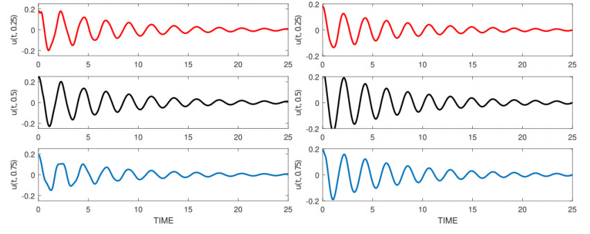
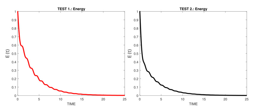
In this work, we consider a viscoelastic wave equation with boundary damping and variable exponents source term. The damping terms and variable exponents are localized on a portion of the boundary. We first, prove the existence of global solutions and then we establish optimal and general decay estimates depending on the relaxation function and the nature of the variable exponent nonlinearity. Finally, we run two numerical tests to demonstrate our theoretical decay results. This study generalizes and enhances existing literature results, and the acquired results are thus of significant importance when compared to previous literature results with constant or variable exponents in the domain.
- variable exponent,
- Lebesgue and Sobolev spaces,
- boundary feedback,
- viscoelasticity,
- relaxation functions,
- general decay,
- finite difference method
Citation: Adel M. Al-Mahdi, Mohammad M. Al-Gharabli, Maher Nour, Mostafa Zahri. Stabilization of a viscoelastic wave equation with boundary damping and variable exponents: Theoretical and numerical study[J]. AIMS Mathematics, 2022, 7(8): 15370-15401. doi: 10.3934/math.2022842

Related Papers:

Abstract

In this work, we consider a viscoelastic wave equation with boundary damping and variable exponents source term. The damping terms and variable exponents are localized on a portion of the boundary. We first, prove the existence of global solutions and then we establish optimal and general decay estimates depending on the relaxation function and the nature of the variable exponent nonlinearity. Finally, we run two numerical tests to demonstrate our theoretical decay results. This study generalizes and enhances existing literature results, and the acquired results are thus of significant importance when compared to previous literature results with constant or variable exponents in the domain.

References

[1]	V. Weston, S. He, Wave splitting of the telegraph equation in r3 and its application to inverse scattering, Inverse Probl., 9 (1993), 789.
[2]	J. Banasiak, J. R. Mika, Singularly perturbed telegraph equations with applications in the random walk theory, J. Appl. Math. Stochastic Anal., 11 (1998), 9–28. https://doi.org/10.1155/S1048953398000021 doi: 10.1155/S1048953398000021
[3]	P. Jordan, A. Puri, Digital signal propagation in dispersive media, J. Appl. Phys., 85 (1999), 1273–1282. https://doi.org/10.1063/1.369258 doi: 10.1063/1.369258
[4]	B. Bulbul, M. Sezer, W. Greiner, Relativistic quantum mechanics wave equations, 2000.
[5]	A. M. Wazwaz, New travelling wave solutions to the boussinesq and the klein-gordon equations, Commun. Nonlinear Sci., 13 (2008), 889–901. https://doi.org/10.1016/j.cnsns.2006.08.005 doi: 10.1016/j.cnsns.2006.08.005
[6]	S. M. El-Sayed, The decomposition method for studying the klein-gordon equation, Chaos Soliton. Fract., 18 (2003), 1025–1030.
[7]	P. Caudrey, J. Eilbeck, J. Gibbon, The sine-gordon equation as a model classical field theory, Il Nuovo. Cimento. B (1971–1996), 25 (1975), 497–512.
[8]	R. K. Dodd, J. C. Eilbeck, J. D. Gibbon, H. C. Morris, Solitons and nonlinear wave equations, 1982.
[9]	J. Perring, T. Skyrme, A model unified field equation, In: Selected Papers, With Commentary, Of Tony Hilton Royle Skyrme, 216–221, World Scientific, 1994.
[10]	G. B. Whitham, Linear and nonlinear waves, John Wiley Sons, 2011.
[11]	A. Ashyralyev, M. E. Köksal, A numerical solution of wave equation arising in non-homogeneous cylindrical shells, Turk. J. Math., 32 (2008), 409–427. https://doi.org/10.1002/uog.6013 doi: 10.1002/uog.6013
[12]	M. E. Koksal, An operator-difference method for telegraph equations arising in transmission lines, Discrete Dyn. Nat. Soc., 2011 (2011).
[13]	W. Chen, R. Ikehata, The cauchy problem for the moore-gibson-thompson equation in the dissipative case, J. Differ. Equations, 292 (2021), 176–219. https://doi.org/10.1002/uog.6013 doi: 10.1002/uog.6013
[14]	W. Chen, A. Palmieri, Nonexistence of global solutions for the semilinear moore-gibson-thompson equation in the conservative case, arXiv preprint arXiv: 1909.08838, 2019.
[15]	W. Chen, T. A. Dao, The cauchy problem for the nonlinear viscous boussinesq equation in the $l^q$ framework, J. Differ. Equations, 320 (2022), 558–597. https://doi.org/10.1016/j.jde.2022.03.001 doi: 10.1016/j.jde.2022.03.001
[16]	A. Ashyralyev, M. E. Koksal, R. P. Agarwal, An operator-difference scheme for abstract cauchy problems, Comput. Math. Appl., 61 (2011), 1855–1872. https://doi.org/10.1016/j.camwa.2011.02.014 doi: 10.1016/j.camwa.2011.02.014
[17]	M. E. Koksal, M. Senol, A. K. Unver, Numerical simulation of power transmission lines, Chinese J. Phys., 59 (2019), 507–524.
[18]	M. E. Koksal, Recent developments on operator-difference schemes for solving nonlocal bvps for the wave equation, Discrete Dyn. Nat. Soc., 2011 (2011).
[19]	A. Ashyralyev, M. E. Koksal, On the numerical solution of hyperbolic pdes with variable space operator, Numer. Meth. Part. D. E., 25 (2009), 1086–1099. https://doi.org/10.1002/num.20388 doi: 10.1002/num.20388
[20]	A. Ashyralyev, M. E. Koksal, Stability of a second order of accuracy difference scheme for hyperbolic equation in a hilbert space, Discrete Dyn. Nat. Soc., 2007 (2007).
[21]	S. Pandit, R. Jiwari, K. Bedi, M. E. Koksal, Haar wavelets operational matrix based algorithm for computational modelling of hyperbolic type wave equations, Eng. Computation., 2017.
[22]	V. Georgiev, G. Todorova, Existence of a solution of the wave equation with nonlinear damping and source terms, J. Differ. Equations, 109 (1994), 295–308. https://doi.org/10.1006/jdeq.1994.1051 doi: 10.1006/jdeq.1994.1051
[23]	H. A. Levine, J. Serrin, A global nonexistence theorem for quasilinear evolution equations with dissipation, 1995.
[24]	E. Vitillaro, Global existence for the wave equation with nonlinear boundary damping and source terms, J. Differ. Equations, 186 (2002), 259–298. https://doi.org/10.1016/S0022-0396(02)00023-2 doi: 10.1016/S0022-0396(02)00023-2
[25]	M. Cavalcanti, V. D. Cavalcanti, J. Prates Filho, J. Soriano, Existence and uniform decay rates for viscoelastic problems with nonlinear boundary damping, Differ. Integral Equ., 14 (2001), 85–116.
[26]	M. M. Al-Gharabli, A. M. Al-Mahdi, S. A. Messaoudi, General and optimal decay result for a viscoelastic problem with nonlinear boundary feedback, J. Dyn. Control Syst., 25 (2019), 551–572. https://doi.org/10.1007/s10883-018-9422-y doi: 10.1007/s10883-018-9422-y
[27]	M. Aassila, A note on the boundary stabilization of a compactly coupled system of wave equations, Appl. Math. Lett., 12 (1999), 19–24.
[28]	H. K. Wang, G. Chen, Asymptotic behaviour of solutions of the one-dimensional wave equation with a nonlinear boundary stabilizer, SIAM J. Control Optim., 27 (1989), 758–775. https://doi.org/10.1137/0327040 doi: 10.1137/0327040
[29]	I. Lasiecka, D. Tataru, Uniform boundary stabilization of semilinear wave equations with nonlinear boundary damping, Differ. Integral Equ., 6 (1993), 507–533.
[30]	E. Zuazua, Uniform stabilization of the wave equation by nonlinear boundary feedback, SIAM J. Control Optim., 28 (1990), 466–477.
[31]	W. Liu, J. Yu, On decay and blow-up of the solution for a viscoelastic wave equation with boundary damping and source terms, Nonlinear Anal-Theor., 74 (2011), 2175–2190. https://doi.org/10.1016/j.na.2010.11.022 doi: 10.1016/j.na.2010.11.022
[32]	M. Ruzicka, Electrorheological fluids: Modeling and mathematical theory, Lect. Notes Math., 1748 (2000), 16–38.
[33]	O. Benslimane, A. Aberqi, J. Bennouna, Existence and uniqueness of weak solution of $ p (x) $-laplacian in sobolev spaces with variable exponents in complete manifolds, arXiv preprint arXiv: 2006.04763, 2020.
[34]	O. A. Omer, M. Z. Abidin, Boundedness of the vector-valued intrinsic square functions on variable exponents herz spaces, Mathematics, 10 (2022), 1168.
[35]	M. A. Ragusa, A. Tachikawa, Regularity of minimizers of some variational integrals with discontinuity, Z. für Anal. und ihre Anwendungen, 27 (2008), 469–482. https://doi.org/10.1002/sim.2928 doi: 10.1002/sim.2928
[36]	S. A. Messaoudi, J. H. Al-Smail, A. A. Talahmeh, Decay for solutions of a nonlinear damped wave equation with variable-exponent nonlinearities, Comput. Math. Appl., 76 (2018), 1863–1875.
[37]	S. Ghegal, I. Hamchi, S. A. Messaoudi, Global existence and stability of a nonlinear wave equation with variable-exponent nonlinearities, Appl. Anal., 99 (2020), 1333–1343.
[38]	S. A. Messaoudi, M. M. Al-Gharabli, A. M. Al-Mahdi, On the decay of solutions of a viscoelastic wave equation with variable sources, Math. Meth. Appl. Sci., 2020.
[39]	M. M. Al-Gharabli, A. M. Al-Mahdi, S. A. Messaoudi, General and optimal decay result for a viscoelastic problem with nonlinear boundary feedback, J. Dyn. Control Syst., 25 (2019), 551–572. https://doi.org/10.1007/s10883-018-9422-y doi: 10.1007/s10883-018-9422-y
[40]	D. Edmunds, J. Rákosník, Sobolev embeddings with variable exponent, Studia Math., 3 (2000), 267–293.
[41]	X. Fan, D. Zhao, On the spaces lp (x)($\omega$) and wm, p (x)($\omega$), J. Math. Anal. Appl., 263 (2001), 424–446.
[42]	L. Diening, P. Harjulehto, P. Hästö, M. Ruzicka, Lebesgue and Sobolev spaces with variable exponents, Springer, 2011.
[43]	M. I. Mustafa, Optimal decay rates for the viscoelastic wave equation, Math. Meth. Appl. Sci., 41 (2018), 192–204. https://doi.org/10.1002/mma.4604 doi: 10.1002/mma.4604
[44]	S. Antontsev, Wave equation with p (x, t)-laplacian and damping term: existence and blow-up, Differ. Equ. Appl., 3 (2011), 503–525.
[45]	L. Lu, S. Li, S. Chai, On a viscoelastic equation with nonlinear boundary damping and source terms: Global existence and decay of the solution, Nonlinear Anal-Real, 12 (2011), 295–303. https://doi.org/10.1016/j.nonrwa.2010.06.016 doi: 10.1016/j.nonrwa.2010.06.016
[46]	S. A. Messaoudi, A. A. Talahmeh, J. H. Al-Smail, Nonlinear damped wave equation: Existence and blow-up, Comput. Math. Appl., 74 (2017), 3024–3041. https://doi.org/10.1016/j.camwa.2017.07.048 doi: 10.1016/j.camwa.2017.07.048
[47]	K. P. Jin, J. Liang, T. J. Xiao, Coupled second order evolution equations with fading memory: Optimal energy decay rate, J. Differ. Equ., 257 (2014), 1501–1528. https://doi.org/10.1016/j.jde.2014.05.018 doi: 10.1016/j.jde.2014.05.018
[48]	V. I. Arnol'd, Mathematical methods of classical mechanics, vol. 60, Springer Science & Business Media, 2013.
[49]	J. H. Hassan, S. A. Messaoudi, M. Zahri, Existence and new general decay results for a viscoelastic timoshenko system, Z. für Anal. und ihre Anwendungen, 39 (2020), 185–222. https://doi.org/10.4171/ZAA/1657 doi: 10.4171/ZAA/1657

Reader Comments

Your name:*

Email:*
© 2022 the Author(s), licensee AIMS Press. This is an open access article distributed under the terms of the Creative Commons Attribution License (http://creativecommons.org/licenses/by/4.0)