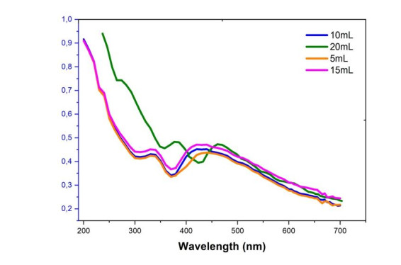
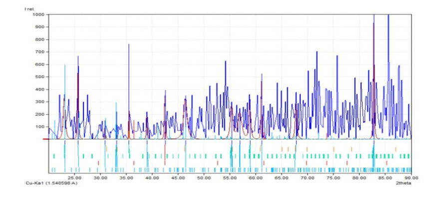
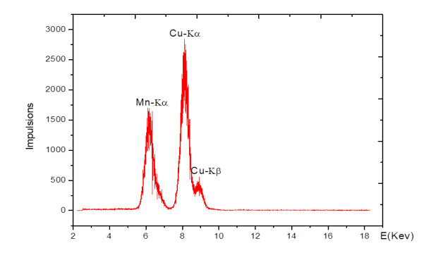
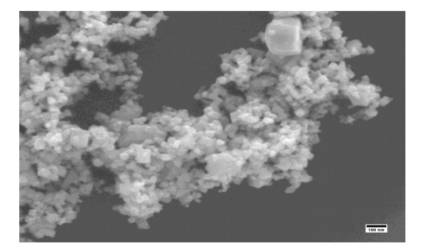
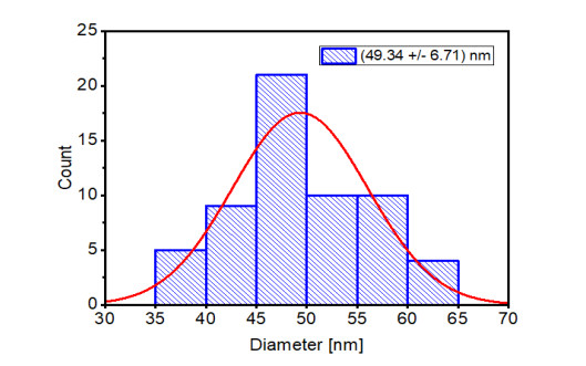
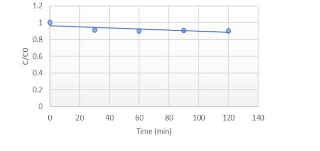
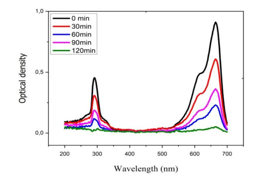
Each year more than 150, 000 tons of dyes are released in effluents by industries. These chemicals entities non-biodegradable and toxic can be removed from effluent by metallic nanomaterials. The aqueous extract of Manotes expansa leaves is used as reducing and stabilizing agent in the biogenic synthesis of Mn-CuO nanocomposites. The nanoparticles obtained were characterized using UV-visible spectroscopy, X-ray Diffraction (XRD), X-ray Fluorescence, Dynamic Light Scattering (DSL), and Scanning Electron Microscopy (SEM). The hemotoxicity of biosynthesized nanomaterials was assessed by evaluating their hemolytic activity using erythrocytes as a model system. The photocatalytic activity of Mn-CuO was carried out by photocatalytic degradation of Methylene Blue dye as a model. The results obtained by UV-vis spectroscopy showed a Plasmonic Surface Resonance band at 408 nm. XRD and X-ray fluorescence made it possible to identify the presence of particles of formula Mn0.53Cu0.21O having crystallized in a Hexagonal system (a = 3.1080 Å and c = 5.2020 Å). Spherical morphology and average height 49.34 ± 6.71 nm were determined by SEM and DSL, respectively. The hemolytic activity of biosynthesized nanomaterials revealed that they are not hemotoxic in vitro (% hemolysis 3.2%) and 98.3% of Methylene Blue dye was removed after 120 min under irradiation with solar light in the presence of Mn-CuO nanocomposites.
Citation: Carlos N. Kabengele, Giresse N. Kasiama, Etienne M. Ngoyi, Clement L. Inkoto, Juvenal M. Bete, Philippe B. Babady, Damien S. T. Tshibangu, Dorothée D. Tshilanda, Hercule M. Kalele, Pius T. Mpiana, Koto-Te-Nyiwa Ngbolua. Biogenic synthesis, characterization and effects of Mn-CuO composite nanocatalysts on Methylene blue photodegradation and Human erythrocytes[J]. AIMS Materials Science, 2023, 10(2): 356-369. doi: 10.3934/matersci.2023019
Each year more than 150, 000 tons of dyes are released in effluents by industries. These chemicals entities non-biodegradable and toxic can be removed from effluent by metallic nanomaterials. The aqueous extract of Manotes expansa leaves is used as reducing and stabilizing agent in the biogenic synthesis of Mn-CuO nanocomposites. The nanoparticles obtained were characterized using UV-visible spectroscopy, X-ray Diffraction (XRD), X-ray Fluorescence, Dynamic Light Scattering (DSL), and Scanning Electron Microscopy (SEM). The hemotoxicity of biosynthesized nanomaterials was assessed by evaluating their hemolytic activity using erythrocytes as a model system. The photocatalytic activity of Mn-CuO was carried out by photocatalytic degradation of Methylene Blue dye as a model. The results obtained by UV-vis spectroscopy showed a Plasmonic Surface Resonance band at 408 nm. XRD and X-ray fluorescence made it possible to identify the presence of particles of formula Mn0.53Cu0.21O having crystallized in a Hexagonal system (a = 3.1080 Å and c = 5.2020 Å). Spherical morphology and average height 49.34 ± 6.71 nm were determined by SEM and DSL, respectively. The hemolytic activity of biosynthesized nanomaterials revealed that they are not hemotoxic in vitro (% hemolysis 3.2%) and 98.3% of Methylene Blue dye was removed after 120 min under irradiation with solar light in the presence of Mn-CuO nanocomposites.

| [1] |
Pinheiro LRS, Gradissimo DG, Xavier LP, et al. (2022) Degradation of azo dyes: Bacterial potential for bioremediation. Sustainability 14: 1510. https://doi.org/10.3390/su14031510. doi: 10.3390/su14031510

|
| [2] |
Rauf MA, Ashraf SS (2009) Review: Fundamental principles and application of heterogeneous photocatalytic degradation of dyes in solution. Chem Eng J 151: 10–18. https://doi.org/10.1016/j.cej.2009.02.026 doi: 10.1016/j.cej.2009.02.026
|
| [3] |
Zhuang Y, Zhu Q, Li G, et al. (2022) Photocatalytic degradation of organic dyes using covalent triazine-based framework. Mater Res Bulletin 146: 111619. https://doi/org/10/1016/j/materresbull.2021.111619. doi: 10.1016/j/materresbull.2021.111619
|
| [4] |
Sibhatu AS, Weldegebrieal KG, Sgaradevan S (2022) Photocatalytic activity of CuO nanoparticles for organic and inorganic pollutants removal in wastewater remediation. Chemosphere 300: 134623. https://doi.org/10.1016/j.chemosphere.2022.134623 doi: 10.1016/j.chemosphere.2022.134623
|
| [5] | Fouda A, Salam S, Wassel AR, et al. (2020) Optimization of green biosynthesized visible light active CuO/ZnO nano-photocatalysts for the degradation of organic methylene blue dye. Hélion 6: e04896. https://doi.org/10.1016/jhelion.2020.e04896. |
| [6] | Lacombe S, Tran-thi T, Guillard C, et al. (2007) La photocalyse pour l'elimination des polluants. Actualités chimique 308: 79–93. |
| [7] |
Liu X, C Chen, Zhao Z, et al. (2013) A review on the synthesis of manganese oxide nanomaterials and their applications on lithium-ion batteries. J Nanomater 2013: 736375. http://dx.doi.org/10.1155/2013/736375 doi: 10.1155/2013/736375
|
| [8] |
Naika HR, Lingaraju K, Manjunath K, et al. (2015) Green synthesis of CuO nanoparticles using Gloriosa superba L. extract and their antibacterial activity. J Taibah Univ Sci 9: 7–12. https://doi.org/10.1016/j.jtusci.2014.04.006. doi: 10.1016/j.jtusci.2014.04.006
|
| [9] |
Ahmad MM, Kotb HM, Mushta S, et al. (2022) Green synthesis of Mn + Cu bimetallic nanoparticles using vinca rosea extract and their antioxidant, antibacterial, and catalytic activities. Crystals 12: 72. https://doi.org/10.3390/cryst12010072. doi: 10.3390/cryst12010072
|
| [10] |
Basavegowda N, Baek K (2021) Multimetallic nanoparticles as alternative antimicrobial agents: Challenges and perspectives. Molecules 26: 912. https://doi.org/10.3390/molecules26040912. doi: 10.3390/molecules26040912
|
| [11] |
Iqbal M, Thebo AA, Shah AH, et al. (2016) Influence of Mn-doping on the photocatalytic and solar cell efficiency of CuO nanowires. Inorg Chem Commun 76: 71–76. https://doi.org/10.1016/j.inoche.2016.11.023. doi: 10.1016/j.inoche.2016.11.023
|
| [12] |
Pramothkumar A, Senthilkumar N, Mercy Gnana Malar KC, et al. (2019) A comparative analysis on the dye degradation efciency of pure, Co, Ni and Mn‑doped CuO nanoparticles. J Mater Sci-Mater El 30: 19043–19059. https://doi.org/10.1007/s10854-019-02262-4. doi: 10.1007/s10854-019-02262-4
|
| [13] | Vindhya PS, Kavitha VT (2022) Leaf extract-mediated synthesis of Mn-doped CuO nanoparticles for antimicrobial, antioxidant and photocatalytic applications. Chem Pap. https://doi.org/10.1007/s11696-022-02631-0. |
| [14] | Kabengele CN, Kasiama GN, Ngoyi EM, et al. (2022) Secondary metabolites and mineral elements of Manotes expansa and Aframomum alboviolaceum leaves collected in the democratic republic of Congo. ARRB 37: 57–63. |
| [15] |
Rizwana H, Alwhibi MS, Al-Judaie RA, et al. (2022) Sunlight-mediated green synthesis of silver nanoparticles using the berries of Ribes rubrum (Red Currants): characterization and evaluation of their antifungal and antibacterial activities. Molecules 27: 2186. https://doi.org/10.3390/molecules27072186. doi: 10.3390/molecules27072186
|
| [16] |
Chen LQ, Li Fang, Ling J, et al. (2015) Nanotoxicity of silver nanoparticles to red blood cells: size dependent adsorption, uptake, and hemolytic activity. Chem Res Toxicol 28: 501–509. https://doi.org/10.1021/tx500479 doi: 10.1021/tx500479
|
| [17] | Pandey S, Singh S (2020) Eco-friendly nanocomposite and properties of manganese nanoparticles using UV-vis and IR fourier spectrum. IJISRT 5: 770–773. |
| [18] |
Shah M, Fawcett D, Sharma S, et al. (2015) Review green synthesis of metallic nanoparticles via biological entities. Materials 8: 7278–7308. https://doi.org/10.3390/ma8115377. doi: 10.3390/ma8115377
|
| [19] | El-seedi, El-Shabasy RM, Khalifa SAM, et al. (2019) Metal nanoparticles fabricated by green chemistry using natural extracts: biosynthesis, mechanisms, and applications. RSC Adv 24539–24559. https://doi.org/10.1039/C9RA02225B |
| [20] |
Makarov VV, Love AJ, Sinitsyna OV, et al. (2014) Green nanotechnologies: Synthesis of metal nanoparticles using plants. Acta Naturae 6: 35–44. https://doi.org/10.32607/20758251-2014-6-1-35-44 doi: 10.32607/20758251-2014-6-1-35-44
|
| [21] |
Desai R, Mankad V, Gupta SG, et al. (2012) Size distribution of silver nanoparticles: UV-visible spectroscopic assessment. Nanosci Nanotechnol Let 4: 30–34. https://doi.org/10.1166/nnl.2012.1278 doi: 10.1166/nnl.2012.1278
|
| [22] |
Yeshchenko OA, Bondarchuk IS, Gurin VS, et al. (2013) Temperature dependence of the surface plasmon resonance in gold nanoparticles. Surf Sci 608: 275–281, http://dx.doi.org/10.1016/j.susc.2012.10.019. doi: 10.1016/j.susc.2012.10.019
|
| [23] |
Seifipour R, Nozari M, Pishkar L (2020) Green synthesis of silver nanoparticles using Tragopogon Collinus leaf extract and study of their antibacterial effects. JIOPM 30: 2926–2936. https://doi.org/10.1007/s10904-020-01441-9 doi: 10.1007/s10904-020-01441-9
|
| [24] |
Vidhu VK, Aromal SA, Philip D (2011) Green synthesis of silver nanoparticles using Macrotyloma uniform. Spectrochim Acta A 83: 392–397. https://doi.org/10.1016/j.saa.2011.08.051 doi: 10.1016/j.saa.2011.08.051
|
| [25] |
Berta L, Coman NA, Rusu A, et al. (2021) A review on plant-Mediated synthesis of Bimetallic nanoparticles, characterization and their biological applications. Materials 14: 7677. https://doi.org/10.3390/ma14247677 doi: 10.3390/ma14247677
|
| [26] |
Pinto VV, Ferreira MJ, Silva R, et al. (2010) Long time effect on the stability of silver nanoparticles in aqueous medium: effect of synthesis and storage conditions. Colloid Surface A 364: 19–25. https://doi.org/10.1016/j.colsurfa.2010.04.015 doi: 10.1016/j.colsurfa.2010.04.015
|
| [27] |
Azeez F, Al-Hetlani E, Arafa M (2018) The effect of surface charge on photocatalytic degradation of Methylene Blue dye using chargeable titania nanoparticles. Sci Rep 2018: 7104. https://doi.org/10.1038/s4158-018-15673-5. doi: 10.1038/s4158-018-15673-5
|
| [28] |
Taylor MG, Augustin N, Gounaris CE, et al. (2015) Catalyst design based on morphology and environment dependent adsorption on metal nanoparticles. ACS Catal 20155: 6296–6301. https://doi.org/10.1021/acscatal.5b01696 doi: 10.1021/acscatal.5b01696
|
| [29] |
Chanu LA, Singh WJ, Singh KJ, et al. (2019) Effect of operational parameters on the photocatalytic degradation of Methylene blue dye solution using manganese doped ZnO nanoparticles. Results Phys 12: 1230–1237. https://doi.org/10.1016/j.rinp.2018.12.089 doi: 10.1016/j.rinp.2018.12.089
|
| [30] |
Dobrovolskaia MA, Clogston JD, Neun BW (2008) Method for analysis of nanoparticle hemolytic properties in vitro. Nano Lett 8: 2180–2187. https://doi.org/10.1021/nl0805615 doi: 10.1021/nl0805615
|
| [31] | Gabor F (2011) Characterization of nanoparticles intended for drug delivery. Sci Pharm 79: 701–702. |
| [32] |
Gul A, Shaheen A, Ahmad I, et al. (2021) Green synthesis, characterization, enzyme inhibition, antimicrobial potential, and cytotoxic activity of plant mediated silver nanoparticle using Ricinus communis leaf and root extracts. Biomolecules 11: 206. https://doi.org/10.3390/biom11020206. doi: 10.3390/biom11020206
|
Figures(11) / Tables(1)

Carlos N. Kabengele, Giresse N. Kasiama, Etienne M. Ngoyi, Clement L. Inkoto, Juvenal M. Bete, Philippe B. Babady, Damien S. T. Tshibangu, Dorothée D. Tshilanda, Hercule M. Kalele, Pius T. Mpiana, Koto-Te-Nyiwa Ngbolua. Biogenic synthesis, characterization and effects of Mn-CuO composite nanocatalysts on Methylene blue photodegradation and Human erythrocytes[J]. AIMS Materials Science, 2023, 10(2): 356-369. doi: 10.3934/matersci.2023019


 DownLoad: