Petrography and structural features of the Precambrian basement rocks in the Benin-Nigerian Shield, NW Nigeria: Implications for their correlation with South Atlantic Precambrian terranes

Emmanuel Daanoba Sunkari; Basiru Mohammed Kore; Samuel Edem Kodzo Tetteh; Emmanuel Daanoba Sunkari; Basiru Mohammed Kore; Samuel Edem Kodzo Tetteh

doi:10.3934/geosci.2022028

AIMS Geosciences

2022, Volume 8, Issue 4: 503-524. doi: 10.3934/geosci.2022028

Previous Article Next Article

Research article

Petrography and structural features of the Precambrian basement rocks in the Benin-Nigerian Shield, NW Nigeria: Implications for their correlation with South Atlantic Precambrian terranes

1.
Department of Geological Engineering, Faculty of Geosciences and Environmental Studies, University of Mines and Technology, P.O. Box 237, Tarkwa, Ghana
2.
Department of Geological Engineering, Faculty of Engineering, Niğde Ömer Halisdemir University, 51240, Main Campus, Niğde, Turkey
3.
Bea Mountain Mining Corporation, Monrovia Office 18^th Street, Payne Avenue Intersection, Monrovia, Liberia

Received: 26 May 2022 Revised: 07 July 2022 Accepted: 02 August 2022 Published: 19 August 2022

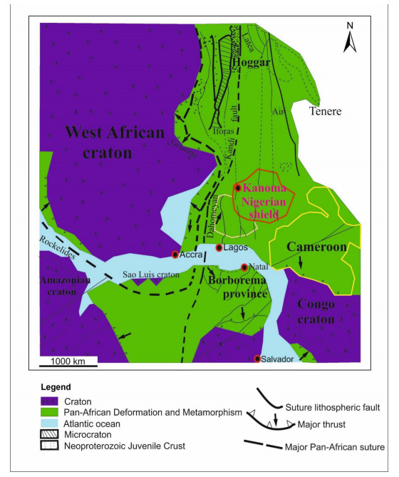
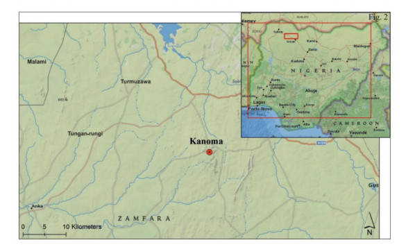
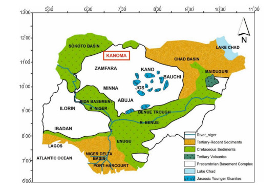
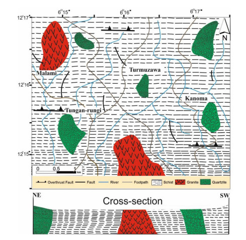
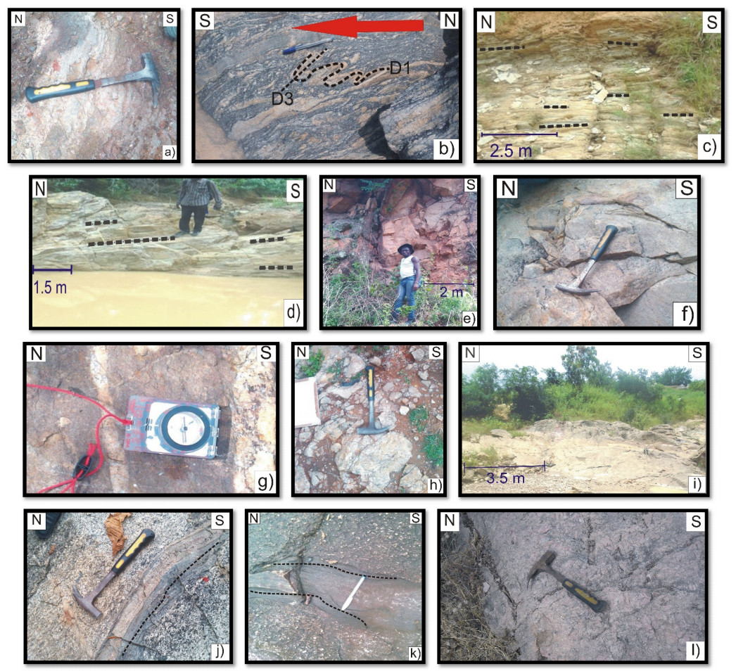
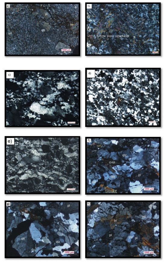
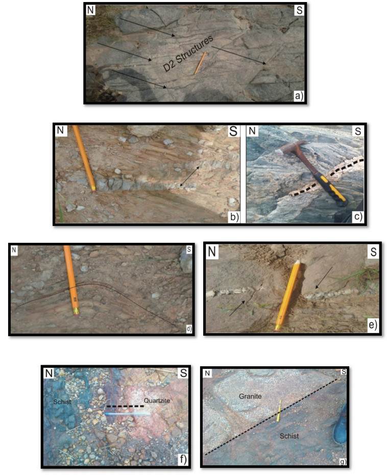
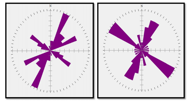
This study investigated the petrographic and structural features of the Precambrian (Neoproterozoic) basement rocks of the Benin-Nigerian Shield that crop out in northwestern Nigeria within Kanoma and its environs to give an insight into the evolution and deformational episodes that pervaded them. The major rock types in the area are schists and quartzites, which have been intruded by granitic rocks that appear to be metamorphosed. The origin of these rocks is attributed to the Eburnean Precambrian orogenic episode and the Pan-African orogeny, which started and ended with the intrusion of the granite suites. The dominant mineralogy associated with the rock types includes quartz, orthoclase, plagioclase, microcline, biotite, chlorite, and very few accessory minerals. The schist shows the dominance of quartz, feldspars (alkali and plagioclase), biotite, muscovite, chlorite, and opaque minerals. The quartzite is typically dominated by quartz that appears recrystallized in places, whereas the meta-granite contains quartz, feldspars (alkali and plagioclase), biotite, and opaque minerals. Structural features such as joints, quartz veins with minor folds, and faults observed in the lithological units have a predominant N-S trend and are the imprints of the last tectonic event (Pan-African orogeny). The level of deformation in Kanoma led to the development of N to NNE trending moderately (S₁) to steeply (S₂) dipping foliations in the schist. The evolution of these deformational mechanisms from moderately dipping foliations to steeply dipping foliations along the N to NNE- trend is associated with late orogenic uplift and exhumation following oblique convergence during the Pan-African orogeny. Structural overprinting relations recognized within Kanoma and its environs allow us to decipher the geologic structures into three successive Pan-African deformational events (D1–D3). D1 fabrics are manifested by simple anticline micro folds in the schist. The D2 structures are the predominant ones in the area comprising the N-S directional joints and faults. The D3 phase of deformation is a progressive one, which started as N-S high angle thrusts and thrust-related folds that resulted from the NE–SW contraction during the orogenic episodes. The studied rocks can be correlated with the Pan-African and Brasiliano belts based on their overlapping features.
- petrography,
- structural evolution,
- Precambrian basement rocks,
- Benin-Nigerian Shield
Citation: Emmanuel Daanoba Sunkari, Basiru Mohammed Kore, Samuel Edem Kodzo Tetteh. Petrography and structural features of the Precambrian basement rocks in the Benin-Nigerian Shield, NW Nigeria: Implications for their correlation with South Atlantic Precambrian terranes[J]. AIMS Geosciences, 2022, 8(4): 503-524. doi: 10.3934/geosci.2022028

Related Papers:

Abstract

This study investigated the petrographic and structural features of the Precambrian (Neoproterozoic) basement rocks of the Benin-Nigerian Shield that crop out in northwestern Nigeria within Kanoma and its environs to give an insight into the evolution and deformational episodes that pervaded them. The major rock types in the area are schists and quartzites, which have been intruded by granitic rocks that appear to be metamorphosed. The origin of these rocks is attributed to the Eburnean Precambrian orogenic episode and the Pan-African orogeny, which started and ended with the intrusion of the granite suites. The dominant mineralogy associated with the rock types includes quartz, orthoclase, plagioclase, microcline, biotite, chlorite, and very few accessory minerals. The schist shows the dominance of quartz, feldspars (alkali and plagioclase), biotite, muscovite, chlorite, and opaque minerals. The quartzite is typically dominated by quartz that appears recrystallized in places, whereas the meta-granite contains quartz, feldspars (alkali and plagioclase), biotite, and opaque minerals. Structural features such as joints, quartz veins with minor folds, and faults observed in the lithological units have a predominant N-S trend and are the imprints of the last tectonic event (Pan-African orogeny). The level of deformation in Kanoma led to the development of N to NNE trending moderately (S₁) to steeply (S₂) dipping foliations in the schist. The evolution of these deformational mechanisms from moderately dipping foliations to steeply dipping foliations along the N to NNE- trend is associated with late orogenic uplift and exhumation following oblique convergence during the Pan-African orogeny. Structural overprinting relations recognized within Kanoma and its environs allow us to decipher the geologic structures into three successive Pan-African deformational events (D1–D3). D1 fabrics are manifested by simple anticline micro folds in the schist. The D2 structures are the predominant ones in the area comprising the N-S directional joints and faults. The D3 phase of deformation is a progressive one, which started as N-S high angle thrusts and thrust-related folds that resulted from the NE–SW contraction during the orogenic episodes. The studied rocks can be correlated with the Pan-African and Brasiliano belts based on their overlapping features.

References

[1]	Egbuniwe IG, Fitches WR, Bentley M, et al. (1985) Late Pan-African syenite-granite plutons in NW Nigeria. J Afr Earth Sci 3: 427-435. doi: 10.1016/S0899-5362(85)80085-3 doi: 10.1016/S0899-5362(85)80085-3
[2]	Caby R (2003) Terrane assembly and geodynamic evolution of central-western Hoggar: a synthesis. J Afr Earth Sci 37: 133-159. doi: 10.1016/j.jafrearsci.2003.05.003 doi: 10.1016/j.jafrearsci.2003.05.003
[3]	Dada SS (2008) Proterozoic evolution of the Nigeria-Boborema province. Geological Society, London, Special Publications, 294: 121-136. doi: 10.1144/SP294.7 doi: 10.1144/SP294.7
[4]	Ganade CE, Cordani UG, Agbossoumounde Y, et al. (2016) Tightening-up NE Brazil and NW Africa connections: New U-Pb/Lu-Hf zircon data of a complete plate tectonic cycle in the Dahomey belt of the West Gondwana Orogen in Togo and Benin. Precambrian Res 276: 24-42. doi: 10.1016/j.precamres.2016.01.032 doi: 10.1016/j.precamres.2016.01.032
[5]	Elatikpo SM, Li H, Zheng H, et al. (2021) Cryogenian crustal evolution in western Nigeria shield: whole-rock geochemistry, Sr-Nd, and zircon U-Pb-Hf isotopic evidence from Bakoshi-Gadanya granites. Int Geol Rev 2021: 1-27. doi: 10.1080/00206814.2021.1998799 doi: 10.1080/00206814.2021.1998799
[6]	Elatikpo SM, Li H, Chen Y, et al. (2022) Genesis and magma fertility of gold-associated high-K granites: LA-ICP-MS zircon trace element and REEs constraint from Bakoshi-Gadanya granites in NW Nigeria. Acta Geochim 41: 351-366. doi: 10.1007/s11631-022-00528-z doi: 10.1007/s11631-022-00528-z
[7]	dos Santos TJS, Fetter AH, Neto JN (2008) Comparisons between the northwestern Borborema Province, NE Brazil, and the southwestern Pharusian Dahomey Belt, SW Central Africa. Geological Society, London, Special Publications, 294: 101-120. doi: 10.1144/SP294.6 doi: 10.1144/SP294.6
[8]	de Lima JV, Guimarães IP, Santos L, et al. (2017) Geochemical and isotopic characterization of the granitic magmatism along the Remígio-Pocinhos shear zone, Borborema Province, NE Brazil. J South Am Earth Sci 75: 116-133. doi: 10.1016/j.jsames.2017.02.004 doi: 10.1016/j.jsames.2017.02.004
[9]	da Costa FG, Klein EL, Lafon JM, et al. (2018) Geochemistry and U-Pb-Hf zircon data for plutonic rocks of the Troia Massif, Borborema Province, NE Brazil: Evidence for reworking of Archean and juvenile Paleoproterozoic crust during Rhyacian accretionary and collisional tectonics. Precambrian Res 311: 167-194. doi: 10.1016/j.precamres.2018.04.008 doi: 10.1016/j.precamres.2018.04.008
[10]	de Lira Santos LCM, Dantas EL, Vidotti RM, et al. (2017) Two-stage terrane assembly in Western Gondwana: Insights from structural geology and geophysical data of central Borborema Province, NE Brazil. J Struct Geol 103: 167-184. doi: 10.1016/j.jsg.2017.09.012 doi: 10.1016/j.jsg.2017.09.012
[11]	Caby R (1989) Precambrian terranes of Benin-Nigeria and northeast Brazil and the Late Proterozoic south Atlantic fit. Geological Society of America Special Papers, 230: 145-158. doi: 10.1130/SPE230-p145 doi: 10.1130/SPE230-p145
[12]	Kennedy Grant N (1970) Geochronology of Precambrian basement rocks from Ibadan, southwestern Nigeria. Earth Planet Sci Lett 10: 29-38. doi: 10.1016/0012-821X(70)90061-0 doi: 10.1016/0012-821X(70)90061-0
[13]	McCurry P (1976) The geology of the Precambrian to Lower Palaeozoic rocks of Northern Nigeria. A review. Geol Nigeria, 15-39.
[14]	Van Breemen O, Pidgeon RT, Bowden P (1977) Age and isotopic studies of some Pan-African granites from North-central Nigeria. Precambrian Res 4: 307-319. doi: 10.1016/0301-9268(77)90001-8 doi: 10.1016/0301-9268(77)90001-8
[15]	Ajibade AC (1982) The origin of the Older Granites of Nigeria: some evidence from the Zungeru region. Niger J Min Geol 19: 223-230.
[16]	Adekoya JA (1996) The Nigerian Schist Belts: Age and depositional environment: Implications from associated banded iron-formations. J Min Geol 31: 35-46.
[17]	Mücke A (2005) The Nigerian manganese-rich iron-formations and their host rocks—from sedimentation to metamorphism. J Afr Earth Sci 41: 407-436. doi: 10.1016/j.jafrearsci.2005.07.003 doi: 10.1016/j.jafrearsci.2005.07.003
[18]	Obaje NG (2009) Geology and Mineral Resources of Nigeria. Dordrecht, Heidelberg, London, New York: Springer-Verlag, 219. doi: 10.1007/978-3-540-92685-6
[19]	Ogungbemi OS, Olatunji O, Oluwatoyin O (2014) Integrated Geophysical Approach to Solid Mineral Exploration: A Case Study of Kusa Mountain, IjeroEkiti, Southwestern Nigeria. Pac J Sci Technol 15: 426-432.
[20]	Ganwa AA, Klötzli US, Diguim Kepnamou A, et al. (2018) Multiple Ediacaran tectono-metamorphic events in the Adamawa-Yadé Domain of the Central Africa Fold Belt: Insight from the zircon U-Pb LAM-ICP-MS geochronology of the metadiorite of Meiganga (Central Cameroon). Geol J 53: 2955-2968. doi: 10.1002/gj.3135 doi: 10.1002/gj.3135
[21]	Odedede O, Ugbe FC (2016) Geochemistry of the gneissic rocks of the basement complex around Kpata, North Central Nigeria. J Appl Geochem 18: 15-21.
[22]	Ogezi AEO (1977) Geochemistry and geochronology of basement rocks from north-western Nigeria. Unpublished Ph.D. Thesis, University of Leeds, 295.
[23]	Adetunji A, Olarewaju VO, Ocan OO, et al. (2018) Geochemistry and U-Pb zircon geochronology of Iwo quartz potassic syenite, southwestern Nigeria: constraints on petrogenesis, timing of deformation and terrane amalgamation. Precambrian Res 307: 125-136. doi: 10.1016/j.precamres.2018.01.015 doi: 10.1016/j.precamres.2018.01.015
[24]	Turner DC (1983) Upper Proterozoic schist belts in the Nigerian sector of the Pan-African province of West Africa. Precambrian Res 21: 55-79. doi: 10.1016/0301-9268(83)90005-0 doi: 10.1016/0301-9268(83)90005-0
[25]	Kröner A, Ekwueme BN, Pidgeon RT (2001) The oldest rocks in West Africa: SHRIMP zircon age for early archean Migmatitic Orthogneiss at Kaduna, Northern Nigeria. J Geol 109: 399-406. doi: 10.1086/319979 doi: 10.1086/319979
[26]	Merdith AS, Collins AS, Williams SE, et al. (2017) A full-plate global reconstruction of the Neoproterozoic. Gondwana Res 50: 84-134. doi: 10.1016/j.gr.2017.04.001 doi: 10.1016/j.gr.2017.04.001
[27]	Ugwuonah EN, Tsunogae T, Obiora SC (2017) Metamorphic P-T evolution of garnet-staurolite-biotite pelitic schist and amphibolite from Keffi, north-central Nigeria: Geothermobarometry, mineral equilibrium modeling, and PT path. J Afr Earth Sci 129: 1-16. doi: 10.1016/j.jafrearsci.2016.12.005 doi: 10.1016/j.jafrearsci.2016.12.005
[28]	Bechiri-Benmerzoug F, Bonin B, Bechiri H, et al. (2017) Hoggar geochronology: a historical review of published isotopic data. Arab J Geosci 10: 1-32. doi: 10.1007/s12517-017-3134-6 doi: 10.1007/s12517-017-3134-6
[29]	Arthaud MH, Caby R, Fuck RA, et al. (2008) Geology of the northern Borborema Province, NE Brazil and its correlation with Nigeria, NW Africa. Geological Society, London, Special Publications, 294: 49-67. doi: 10.1144/SP294.4 doi: 10.1144/SP294.4
[30]	Annor AE (1995) U-Pb zircon age for Kabba-Okene granodiorite gneiss: implication for Nigeria's basement chronology. Afr Geosci Rev 2: 101-105.
[31]	Okonkwo CT, Ganev VY (2012) U-Pb Geochronology of the Jebba granitic gneiss and its implications for the Paleoproterozoic evolution of Jebba area, southwestern Nigeria. Int J Geosci 3: 1065-1073. http://dx.doi.org/10.4236/ijg.2012.35107 doi: 10.4236/ijg.2012.35107
[32]	Neves SP (2003) Proterozoic history of the Borborema province (NE Brazil): Correlations with neighboring cratons and Pan-African belts and implications for the evolution of western Gondwana. Tectonics 22: 10-31. doi: 10.1029/2001TC001352 doi: 10.1029/2001TC001352
[33]	Van Schmus WR, Oliveira EP, da Silva Filho AF, et al. (2008) Proterozoic links between the Borborema province, NE Brazil, and the central African fold belt. Geological Society, London, Special Publications, 294: 69-99. doi: 10.1144/SP294.5 doi: 10.1144/SP294.5
[34]	Ledru P, Johan V, Milési JP, et al. (1994) Markers of the last stages of the Palaeoproterozoic collision: evidence for a 2 Ga continent involving circum-South Atlantic provinces. Precambrian Res 69: 169-191. doi: 10.1016/0301-9268(94)90085-X doi: 10.1016/0301-9268(94)90085-X
[35]	Ngako V, Njonfang E (2011) Plates amalgamation and plate destruction, the Western Gondwana history. In Closson D, eds, Tectonics, 358.
[36]	Norcross C, Davis DW, Spooner ET, et al. (2000) U-Pb and Pb-Pb age constraints on Paleoproterozoic magmatism, deformation and gold mineralization in the Omai area, Guyana Shield. Precambrian Res 102: 69-86. doi: 10.1016/S0301-9268(99)00102-3 doi: 10.1016/S0301-9268(99)00102-3
[37]	Rogers JJW (1996) A history of continents in the past three billion years. J Geol 104: 91-107. doi: 10.1086/629803 doi: 10.1086/629803
[38]	Mariano G, Neves SP, Da Siva Filho AF, et al. (2001) Diorites of the high-K calc-alkalic association: geochemistry and Sm-Nd data and implications for the evolution of the Borborema Province, Northeast Brazil. Int Geol Rev 43: 921-929. doi: 10.1080/00206810109465056 doi: 10.1080/00206810109465056

Reader Comments

Your name:*

Email:*
© 2022 the Author(s), licensee AIMS Press. This is an open access article distributed under the terms of the Creative Commons Attribution License (http://creativecommons.org/licenses/by/4.0)