Onset of triple-diffusive convective stability in the presence of a heat source and temperature gradients: An exact method

Yellamma; N. Manjunatha; Umair Khan; Samia Elattar; Sayed M. Eldin; Jasgurpreet Singh Chohan; R. Sumithra; K. Sarada; Yellamma; N. Manjunatha; Umair Khan; Samia Elattar; Sayed M. Eldin; Jasgurpreet Singh Chohan; R. Sumithra; K. Sarada

doi:10.3934/math.2023681

AIMS Mathematics

2023, Volume 8, Issue 6: 13432-13453. doi: 10.3934/math.2023681

Previous Article Next Article

Research article Special Issues

Onset of triple-diffusive convective stability in the presence of a heat source and temperature gradients: An exact method

1.
Department of Mathematics, School of Applied Sciences, REVA University, Bengaluru-560064, India
2.
Department of Mathematical Sciences, Faculty of Science and Technology, Universiti Kebangsaan Malaysia, UKM Bangi 43600, Selangor, Malaysia
3.
Department of Mathematics and Social Sciences, Sukkur IBA University, Sukkur 65200, Sindh Pakistan
4.
Department of Industrial and Systems Engineering, College of Engineering, Princess Nourah bint Abdulrahman University, P.O. Box 84428, Riyadh 11671, Saudi Arabia
5.
Center of Research, Faculty of Engineering, Future University in Egypt, New Cairo 11835, Egypt
6.
Department of Mechanical Engineering and University Centre for Research and Development, Chandigarh University, Mohali-140413, India
7.
Department of UG, PG Studies and Research in Mathematics, Nrupathunga University, Bengaluru-560001, India
8.
Department of Mathematics, Government City College, Hyderabad, India

Received: 05 January 2023 Revised: 17 February 2023 Accepted: 01 March 2023 Published: 06 April 2023
MSC : 76Rxx, 76R05, 80M30

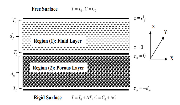
In the current work, in the presence of a heat source and temperature gradients, the onset of triple-diffusive convective stability is studied for a fluid, and a fluid-saturated porous layer confined vertically by adiabatic limits for the Darcy model is thoroughly analyzed. With consistent heat sources in both layers, this composite layer is subjected to three temperature profiles with Marangoni effects. The fluid-saturated porous region's lower boundary is a rigid surface, while the fluid region's upper boundary is a free surface. For the system of ordinary differential equations, the thermal surface-tension-driven (Marangoni) number, which also happens to be the Eigenvalue, is solved in closed form. The three different temperature profiles are investigated, the thermal surface-tension-driven (Marangoni) numbers are calculated analytically, and the effects of the heat source/sink are studied in terms of corrected internal Rayleigh numbers. Graphs are used to show how different parameters have an impact on the onset of triple-diffusive convection. The study's parameters have a greater influence on porous layer dominant composite layer systems than on fluid layer dominant composite layer systems. Finally, porous parameters and corrected internal Rayleigh numbers are stabilize the system, and solute1 Marangoni number and ratio of solute2 diffusivity to thermal diffusivity of fluid are destabilize the system.
- triple-diffusive,
- convective stability,
- adiabatic boundaries,
- composite layer,
- heat source/sink,
- thermal Marangoni number
Citation: Yellamma, N. Manjunatha, Umair Khan, Samia Elattar, Sayed M. Eldin, Jasgurpreet Singh Chohan, R. Sumithra, K. Sarada. Onset of triple-diffusive convective stability in the presence of a heat source and temperature gradients: An exact method[J]. AIMS Mathematics, 2023, 8(6): 13432-13453. doi: 10.3934/math.2023681

Related Papers:

Abstract

In the current work, in the presence of a heat source and temperature gradients, the onset of triple-diffusive convective stability is studied for a fluid, and a fluid-saturated porous layer confined vertically by adiabatic limits for the Darcy model is thoroughly analyzed. With consistent heat sources in both layers, this composite layer is subjected to three temperature profiles with Marangoni effects. The fluid-saturated porous region's lower boundary is a rigid surface, while the fluid region's upper boundary is a free surface. For the system of ordinary differential equations, the thermal surface-tension-driven (Marangoni) number, which also happens to be the Eigenvalue, is solved in closed form. The three different temperature profiles are investigated, the thermal surface-tension-driven (Marangoni) numbers are calculated analytically, and the effects of the heat source/sink are studied in terms of corrected internal Rayleigh numbers. Graphs are used to show how different parameters have an impact on the onset of triple-diffusive convection. The study's parameters have a greater influence on porous layer dominant composite layer systems than on fluid layer dominant composite layer systems. Finally, porous parameters and corrected internal Rayleigh numbers are stabilize the system, and solute1 Marangoni number and ratio of solute2 diffusivity to thermal diffusivity of fluid are destabilize the system.

References

[1]	E. T. Degens, R. P. Von Herzen, H. K. Wong, W. G. Deuser, H. W. Jannasch, Lake Kivu: Structure, chemistry and biology of an east African rift lake, Geol. Rundsch., 62 (1973), 245−277. https://doi.org/10.1007/BF01826830 doi: 10.1007/BF01826830
[2]	R. Sumithra, Exact solution of triple diffusive Marangoni convection in a composite layer, Inter. J. Eng. Res. Tech., 1 (2012), 1−13.
[3]	I. S. Shivakumara, S. B. Naveen Kumar, Linear and weakly nonlinear triple diffusive convection in a couple stress fluid layer, Int. J. Heat Mass Tran., 68 (2014), 542−553. https://doi.org/10.1016/j.ijheatmasstransfer.2013.09.051 doi: 10.1016/j.ijheatmasstransfer.2013.09.051
[4]	G. C. Rana, R. Chand, V. Sharma, A. Sharda, On the onset of triple-diffusive convection in a layer of nanofluid, J. Comput. Appl. Mech., 47 (2016), 67−77. https://doi.org/10.22059/JCAMECH.2016.59256 doi: 10.22059/JCAMECH.2016.59256
[5]	K. R. Raghunatha, I. S. Shivakumara, B. M. Shankar, Weakly nonlinear stability analysis of triple diffusive convection in a Maxwell fluid saturated porous layer, Appl. Math. Mech., 39 (2018), 153−168. https://doi.org/10.1007/s10483-018-2298-6 doi: 10.1007/s10483-018-2298-6
[6]	P. M. Patil, Monisha Roy, S. Roy, E. Momoniat, Triple diffusive mixed convection along a vertically moving surface, Int. J. Heat Mass Tran., 117 (2018), 287−295. https://doi.org/10.1016/j.ijheatmasstransfer.2017.09.106 doi: 10.1016/j.ijheatmasstransfer.2017.09.106
[7]	P. M. Patil, M. Roy, A. Shashikant, S. Roy, E. Momoniat, Triple diffusive mixed convection from an exponentially decreasing mainstream velocity, Int. J. Heat Mass Tran., 124 (2018), 298−306. https://doi.org/10.1016/j.ijheatmasstransfer.2018.03.052 doi: 10.1016/j.ijheatmasstransfer.2018.03.052
[8]	G. Melathil, S. Pranesh, S. Tarannum, Effects of magnetic field and internal heat generation on triple diffusive convection in an Oldroyd-B liquid, Int. J. Res. Advent Tech., 7 (2019), 154−163.
[9]	M. Archana, B. J. Gireesha, B. C. Prasannakumara, Triple diffusive flow of Casson nanofluid with buoyancy forces and nonlinear thermal radiation over a horizontal plate, Arch. Thermodyn., 40 (2019), 49–69. https://doi.org/10.24425/ather.2019.128289 doi: 10.24425/ather.2019.128289
[10]	I. A. Badruddin, Azeem, T. M. Yunus Khan, M. A. Ali Baig, Heat transfer in porous media: A mini review, Mater. Today, 24 (2020), 1318−1321. https://doi.org/10.1016/j.matpr.2020.04.447 doi: 10.1016/j.matpr.2020.04.447
[11]	S. U. Khan, H. Vaidya, W. Chammam, S. A. Musmar, K. V. Prasad, I. Tlili, Triple diffusive unsteady flow of Eyring-Powell nanofluid over a periodically accelerated surface with variable thermal features, Front. Phys., 8 (2020), 246. https://doi.org/10.3389/fphy.2020.00246 doi: 10.3389/fphy.2020.00246
[12]	S. Shankar, S. B. Ramakrishna, N. Gullapalli, N. Samuel, Triple diffusive MHD Casson fluid flow over a vertical wall with convective boundary conditions, Biointerface Res. Appl. Chem., 11 (2021), 13765−13778. https://doi.org/10.33263/BRIAC116.1376513778 doi: 10.33263/BRIAC116.1376513778
[13]	Y. X. Li, U. F. Alqsair, K. Ramesh, S. U. Khan, M. I. Khan, Nonlinear heat source/sink and activation energy assessment in double diffusion flow of micropolar (non-Newtonian) nanofluid with convective conditions, Arab J. Sci. Eng., 47 (2022), 859–866. https://doi.org/10.1007/s13369-021-05692-7 doi: 10.1007/s13369-021-05692-7
[14]	M. Sohail, U. Nazir, E. R. El-Zahar, H. Alrabaiah, P. Kumam, A. A. A. Mousa, et al., A study of triple-mass diffusion species and energy transfer in Carreau–Yasuda material influenced by activation energy and heat source, Sci. Rep., 12 (2022), 10219. https://doi.org/10.1038/s41598-022-13890-y doi: 10.1038/s41598-022-13890-y
[15]	B. K. Sharma, R. Gandhi, Combined effects of Joule heating and non-uniform heat source/sink on unsteady MHD mixed convective flow over a vertical stretching surface embedded in a Darcy-Forchheimer porous medium, Propul. Power Res., 11 (2022), 276−292. https://doi.org/10.1016/j.jppr.2022.06.001 doi: 10.1016/j.jppr.2022.06.001
[16]	S. Noor Arshika, S. Tarannum, S. Pranesh, Heat and mass transfer of triple diffusive convection in viscoelastic liquids under internal heat source modulations, Heat Tran., 51 (2022), 239−256. https://doi.org/10.1002/htj.22305 doi: 10.1002/htj.22305
[17]	V. Nagendramma, P. Durgaprasad, N. Sivakumar, B. M. Rao, C. S. K. Raju, N. A. Shah, S. J. Yook, Dynamics of triple diffusive free convective MHD fluid flow: Lie group transformation, Mathematics, 10 (2022), 2456. https://doi.org/10.3390/math10142456 doi: 10.3390/math10142456
[18]	J. V. Ramana Reddy, K. Anantha Kumar, V. Sugunamma, N. Sandeep, Effect of cross diffusion on MHD non-Newtonian fluids flow past a stretching sheet with non-uniform heat source/sink: A comparative study, Alex. Eng. J., 57 (2018), 1829−1838. https://doi.org/10.1016/j.aej.2017.03.008 doi: 10.1016/j.aej.2017.03.008
[19]	B. J. Gireesha, K. Ganesh Kumar, G. K. Ramesh, B. C. Prasannakumara, Nonlinear convective heat and mass transfer of Oldroyd-B nanofluid over a stretching sheet in the presence of uniform heat source/sink, Results Phys., 9 (2018), 1555−1563. https://doi.org/10.1016/j.rinp.2018.04.006 doi: 10.1016/j.rinp.2018.04.006
[20]	N. Sandeep, C. Sulochana, Momentum and heat transfer behaviour of Jeffrey, Maxwell and Oldroyd-B nanofluids past a stretching surface with non-uniform heat source/sink, Ain Shams Eng. J., 9 (2018), 517−524. https://doi.org/10.1016/j.asej.2016.02.008 doi: 10.1016/j.asej.2016.02.008
[21]	K. E. Aslani, U. S. Mahabaleshwar, P. H. Sakanaka, I. E. Sarris, Effect of partial slip and radiation on liquid film fluid flow over an unsteady porous stretching sheet with viscous dissipation and heat source/sink, J. Porous Media, 24 (2021), 1−15. https://doi.org/10.1615/JPorMedia.2021035873 doi: 10.1615/JPorMedia.2021035873
[22]	R. J. Punith Gowda, R. Naveen Kumar, A. M. Jyothi, B. C. Prasannakumara, I. E. Sarris, Impact of binary chemical reaction and activation energy on heat and mass transfer of Marangoni driven boundary layer flow of a non-Newtonian nanofluid, Processes, 9 (2021), 702. https://doi.org/10.3390/pr9040702 doi: 10.3390/pr9040702
[23]	M. Ibrahim, T. Saeed, F. Riahi Bani, S. N. Sedeh, Y. M. Chu, D. Toghraie, Two-phase analysis of heat transfer and entropy generation of water-based magnetite nanofluid flow in a circular micro tube with twisted porous blocks under a uniform magnetic field, Powder Technol., 384 (2021), 522−541. https://doi.org/10.1016/j.powtec.2021.01.077 doi: 10.1016/j.powtec.2021.01.077
[24]	K. Sajjan, N. Ameer Ahammad, C. S. K. Raju, N. A. Shah, T. Botmart, Study of nonlinear thermal convection of ternary nanofluid within Darcy-Brinkman porous structure with time dependent heat source/sink, AIMS Mathematics, 8 (2023), 4237–4260. https://doi.org/ 10.3934/math.2023211 doi: 10.3934/math.2023211
[25]	T. Mahesh Kumar, N. A. Shah, V. Nagendramma, P. Durgaprasad, N. Sivakumar, B. Madhusudhana Rao, et al., Linear regression of triple diffusive and dual slip flow using Lie Group transformation with and without hydro-magnetic flow, AIMS Mathematics, 8 (2023), 5950–5979. https://doi.org/10.3934/math.2023300 doi: 10.3934/math.2023300
[26]	S. U. Mamatha, R. L. V. Renuka Devi, N. Ameer Ahammad, N. A. Shah, B. Madhusudhan Rao, C. S. K. Raju, et al., Multi-linear regression of triple diffusive convectively heated boundary layer flow with suction and injection: Lie group transformations, Int. J. Mod. Phys. B, 37 (2023), 2350007. https://doi.org/10.1142/S0217979223500078 doi: 10.1142/S0217979223500078
[27]	T. Liu, Reconstruction of a permeability field with the wavelet multiscale-homotopy method for a nonlinear convection-diffusion equation, Appl. Math. Comput., 275 (2016), 432–437. https://doi.org/10.1016/j.amc.2015.11.095 doi: 10.1016/j.amc.2015.11.095
[28]	T. Liu, Porosity reconstruction based on Biot elastic model of porous media by homotopy perturbation method, Chaos Solitons Fractals, 158 (2022), 112007. https://doi.org/10.1016/j.chaos.2022.112007 doi: 10.1016/j.chaos.2022.112007
[29]	N. Manjunatha, R. Sumithra, Effects of non-uniform temperature gradients on triple diffusive surface tension driven magneto convection in a composite layer, Univer. J. Mech. Eng., 7 (2019), 398–410. https://doi.org/10.13189/ujme.2019.070611 doi: 10.13189/ujme.2019.070611
[30]	N. Manjunatha, R. Sumithra, Triple diffusive surface tension driven convection in a composite layer in the presence of vertical magnetic field, Int. J. Eng. Adv. Tech., 9 (2020), 1727–1734. https://doi.org/10.35940/ijeat.C5707.029320 doi: 10.35940/ijeat.C5707.029320
[31]	N. Manjunatha, R. Sumithra, Effects of heat source/sink on Darcian-Bènard-Magneto-Marangoni convection in a composite layer subjected to non-uniform temperature gradients, TWMS J. Appl. Eng. Math., 12 (2022), 669–684.
[32]	N. Manjunatha, R. Sumithra, R. K. Vanishree, Influence of constant heat source/sink on non-Darcian-Bènard double diffusive Marangoni convection in a composite layer system, J. Appl. Math. Inform., 40 (2022), 99–115. https://doi.org/10.14317/jami.2022.099 doi: 10.14317/jami.2022.099
[33]	P. Rudolph, W. Wang, K. Tsukamoto, D. Wu, Transport phenomena of crystal growth-heat and mass transfer, AIP Conf. Proc. 1270 (2010), 107–132. https://doi.org/10.1063/1.3476222 doi: 10.1063/1.3476222
[34]	P. H. Roberts, Electrohydrodynamic convection, Q. J. Mech. Appl. Math., 22 (1969), 211–220. https://doi.org/10.1093/qjmam/22.2.211 doi: 10.1093/qjmam/22.2.211
[35]	M. I. Char, K. T. Chiang, Boundary effects on the Bènard-Marangoni instability under an electric field, Appl. Sci. Res., 52 (1994), 331–354. https://doi.org/10.1007/BF00936836 doi: 10.1007/BF00936836
[36]	J. A. Del Rio, S. Whitaker, Electrohydrodynamics in porous media, Transp. Porous Media, 440 (2001), 385–405. https://doi.org/10.1023/A:1010762226382 doi: 10.1023/A:1010762226382
[37]	M. I. Othman, Electrohydrodynamic instability of a rotating layer of a viscoelastic fluid heated from below, Z. Angew. Math. Phys., 55 (2004), 468–482. https://doi.org/10.1007/s00033-003-1156-2 doi: 10.1007/s00033-003-1156-2
[38]	I. S. Shivakumara, N. Rudraiah, C. E. Nanjundappa., Effect of non-uniform basic temperature gradient on Rayleigh-Bènard-Marangoni convection in ferrofluids, J. Magn. Magn. Mater., 248 (2002), 379–395. https://doi.org/10.1016/S0304-8853(02)00151-8 doi: 10.1016/S0304-8853(02)00151-8
[39]	I. S. Shivakumara, S. Suma, K. B. Chavaraddi, Onset of surface tension driven convection in superposed layers of fluid and saturated porous medium, Arch. Mech., 58 (2006), 71–92.
[40]	I. S. Shivakumara, S. Suresh Kumar, N. Devaraju, Effect of non-uniform temperature gradients on the onset of convection in a couple-stress fluid-saturated porous medium, J. Appl. Fluid. Mech., 5 (2012), 49–55. https://doi.org/10.36884/jafm.5.01.11957 doi: 10.36884/jafm.5.01.11957
[41]	P. N. Kaloni, J. X. Lou, Convective instability of magnetic fluids, Phys. Rev. E, 70 (2004), 026313. https://doi.org/10.1103/PhysRevE.70.026313 doi: 10.1103/PhysRevE.70.026313
[42]	E. W. Sparrow, R. J. Goldstein, V. K. Jonson, Thermal instability in a horizontal fluid layer effect of boundary conditions and non-linear temperature profile, J. Fluid Mech., 18 (1964), 513–528. https://doi.org/10.1017/S0022112064000386 doi: 10.1017/S0022112064000386

Reader Comments

Your name:*

Email:*
© 2023 the Author(s), licensee AIMS Press. This is an open access article distributed under the terms of the Creative Commons Attribution License (http://creativecommons.org/licenses/by/4.0)