Can synoptic patterns influence the track and formation of tropical cyclones in the Mozambique Channel?

Chibuike Chiedozie Ibebuchi; Chibuike Chiedozie Ibebuchi

doi:10.3934/geosci.2022003

AIMS Geosciences

2022, Volume 8, Issue 1: 33-51. doi: 10.3934/geosci.2022003

Previous Article Next Article

Research article

Can synoptic patterns influence the track and formation of tropical cyclones in the Mozambique Channel?

Chibuike Chiedozie Ibebuchi ^,

Institute of Geography and Geology, University of Würzburg, Am Hubland, 97074 Würzburg, Germany

Received: 17 October 2021 Revised: 06 January 2022 Accepted: 10 January 2022 Published: 14 January 2022

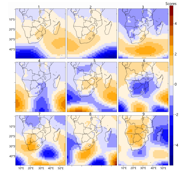
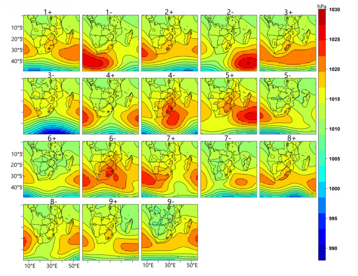
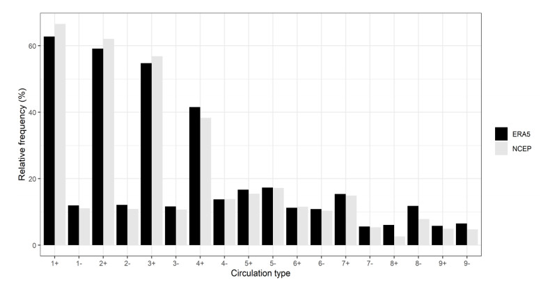
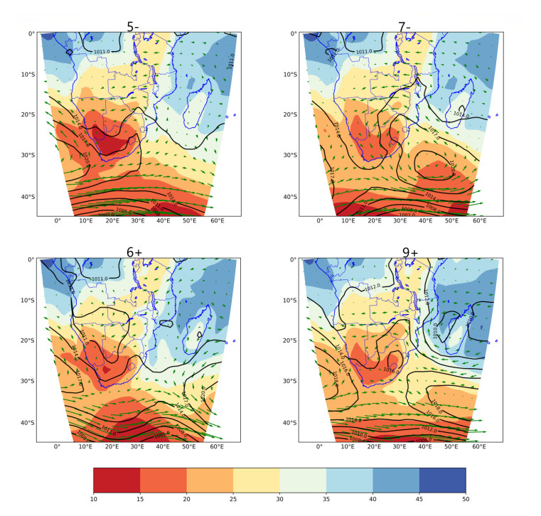
The influence of large-scale circulation patterns on the track and formation of tropical cyclones (TCs) in the Mozambique Channel is investigated in this paper. The output of the hourly classification of circulation types (CTs), in Africa, south of the equator, using rotated principal component analysis on the T-mode matrix (variable is time series and observation is grid points) of sea level pressure (SLP) from ERA5 reanalysis from 2010 to 2019 was used to investigate the time development of the CTs at a sub-daily scale. The result showed that at specific seasons, certain CTs are dominant so that their features overlap with other CTs. CTs with synoptic features, such as enhanced precipitable water and cyclonic activity in the Mozambique Channel that can be favorable for the development of TC in the Channel were noted. The 2019 TC season in the Mozambique Channel characterized by TC Idai in March and TC Kenneth afterward in April were used in evaluating how the CTs designated to have TC characteristics played role in the formation and track of the TCs towards their maximum intensity. The results were discussed and it generally showed that large-scale circulation patterns can influence the formation and track of the TCs in the Mozambique Channel especially through (ⅰ) variations in the position and strength of the anticyclonic circulation at the western branch of the Mascarene high; (ⅱ) modulation of wind speed and wind direction; hence influencing convergence in the Channel; (ⅲ) and modulation of the intensity of cyclonic activity in the Channel that can influence large-scale convection.
- circulation type,
- tropical cyclones,
- hourly classification,
- Mozambique Channel,
- Africa south of the equator
Citation: Chibuike Chiedozie Ibebuchi. Can synoptic patterns influence the track and formation of tropical cyclones in the Mozambique Channel?[J]. AIMS Geosciences, 2022, 8(1): 33-51. doi: 10.3934/geosci.2022003

Related Papers:

Abstract

The influence of large-scale circulation patterns on the track and formation of tropical cyclones (TCs) in the Mozambique Channel is investigated in this paper. The output of the hourly classification of circulation types (CTs), in Africa, south of the equator, using rotated principal component analysis on the T-mode matrix (variable is time series and observation is grid points) of sea level pressure (SLP) from ERA5 reanalysis from 2010 to 2019 was used to investigate the time development of the CTs at a sub-daily scale. The result showed that at specific seasons, certain CTs are dominant so that their features overlap with other CTs. CTs with synoptic features, such as enhanced precipitable water and cyclonic activity in the Mozambique Channel that can be favorable for the development of TC in the Channel were noted. The 2019 TC season in the Mozambique Channel characterized by TC Idai in March and TC Kenneth afterward in April were used in evaluating how the CTs designated to have TC characteristics played role in the formation and track of the TCs towards their maximum intensity. The results were discussed and it generally showed that large-scale circulation patterns can influence the formation and track of the TCs in the Mozambique Channel especially through (ⅰ) variations in the position and strength of the anticyclonic circulation at the western branch of the Mascarene high; (ⅱ) modulation of wind speed and wind direction; hence influencing convergence in the Channel; (ⅲ) and modulation of the intensity of cyclonic activity in the Channel that can influence large-scale convection.

References

[1]	Harr AP, Elsberry RL (1995) Large-scale circulation variability over the Tropical Western North Pacific. Part 1: spatial patterns and tropical cyclone characteristics. Mon Weather Rev 123: 1225-1246. https://doi.org/10.1175/1520-0493(1995)123<1225:LSCVOT>2.0.CO;2 doi: 10.1175/1520-0493(1995)123<1225:LSCVOT>2.0.CO;2
[2]	Jury MR (1993) A preliminary study of climatological associations and characteristics of tropical cyclones in the SW Indian Ocean. Meteorl Atmos Phys 51: 101-115. https://doi.org/10.1007/BF01080882 doi: 10.1007/BF01080882
[3]	Ibebuchi CC (2021) Circulation pattern controls of wet days and dry days in Free State, South Africa. Meteorol Atmos Phys 133: 1469-1480. https://doi.org/10.1007/s00703-021-00822-0 doi: 10.1007/s00703-021-00822-0
[4]	Smith RK (2006) Lectures on tropical cyclones. Available from: https://www.meteo.physik.uni-muenchen.de/~roger/Lectures/Tropical_Cyclones/060510_tropical_cyclones.pdf
[5]	Varotsos CA, Efstathiou MN (2013) Is there any long-term memory effect in the tropical cyclones? Theor Appl Climatol 114: 643-650. https://doi.org/10.1007/s00704-013-0875-3 doi: 10.1007/s00704-013-0875-3
[6]	Ash KC, Matyas J (2012) The inﬂuences of ENSO and the Subtropical Indian Ocean Dipole on tropical cyclone trajectories in the South Indian Ocean. Int J Climatol 32: 41-56. https://doi.org/10.1002/joc.2249 doi: 10.1002/joc.2249
[7]	Pillay MT, Fitchett JM (2019) Tropical cyclone landfalls south of the Tropic of Capricorn, southwest Indian Ocean. Clim Res 79: 23-37. https://doi.org/10.3354/cr01575 doi: 10.3354/cr01575
[8]	Varotsos CA, Efstathiou MN, Cracknell AP (2015) Sharp rise in hurricane and cyclone count during the last century. Theor Appl Climatol 119: 629-638. https://doi.org/10.1007/s00704-014-1136-9 doi: 10.1007/s00704-014-1136-9
[9]	Oguejiofor CN, Abiodun BJ (2019) Simulating the influence of sea-surface-temperature (SST) on tropical cyclones over South-West Indian ocean, using the UEMS-WRF regional climate model. arXiv Atmos Oceanic Phys.
[10]	Gray WM (1968) Global view of the origin of tropical disturbances and storms. Mon Weather Rev 96: 669-700. https://doi.org/10.1175/1520-0493(1968)096<0669:GVOTOO>2.0.CO;2 doi: 10.1175/1520-0493(1968)096<0669:GVOTOO>2.0.CO;2
[11]	Fitchett JM (2018) Recent emergence of CAT5 tropical cyclones in the South Indian Ocean. S Afr J Sci 114: 1-6. https://doi.org/10.17159/sajs.2018/4426 doi: 10.17159/sajs.2018/4426
[12]	Muthige MS, Malherbe J, Englebrecht FA, et al. (2018) Projected changes in tropical cyclones over the South West Indian Ocean under different extents of global warming. Environ Res Lett 13: 065019.
[13]	Malherbe J, Engelbrecht FA, Landman WA (2013) Projected changes in tropical cyclone climatology and landfall in the Southwest Indian Ocean region under enhanced anthropogenic forcing. Clim Dyn 40: 2867-2886. https://doi.org/10.1007/s00382-012-1635-2 doi: 10.1007/s00382-012-1635-2
[14]	Pillay MT, Fitchett JM (2020) Southern hemisphere tropical cyclones: A critical analysis of regional characteristics. Int J Climatol 41: 146-161. https://doi.org/10.1002/joc.6613 doi: 10.1002/joc.6613
[15]	Jury MR, Pathack B (1991) A study of climate and weather variability over the tropical Southwest Indian Ocean. Meteorl Atmos Phys 47: 37-48. https://doi.org/10.1007/BF01025825 doi: 10.1007/BF01025825
[16]	Malan N, Reason CJC, Loveday BR (2013) Variability in tropical cyclone heat potential over the Southwest Indian Ocean. J Geophys Res Oceans 118: 6734-6746. https://doi.org/10.1002/2013JC008958 doi: 10.1002/2013JC008958
[17]	Malherbe J, Engelbrecht F, Landman W, et al. (2011) High resolution model projections of tropical cyclone landfall over southern Africa under enhanced anthropogenic forcing. South African Society for Atmospheric Sciences 27th Annual Conference, 22-23. http://hdl.handle.net/10204/5680
[18]	Klinman MG, Reason CJC (2008) On the peculiar storm track of TC Favio during the 2006-2007 Southwest Indian Ocean tropical cyclone season and relationships to ENSO. Meteorol Atmos Phys 100: 233-242. https://doi.org/10.1007/s00703-008-0306-7 doi: 10.1007/s00703-008-0306-7
[19]	Xulu NG, Chikoore H, Bopape MJM, et al. (2020) Climatology of the Mascarene High and its influence on weather and climate over southern Africa. Climate 8: 86. https://doi.org/10.3390/cli8070086 doi: 10.3390/cli8070086
[20]	Reason CJC (2002) Sensitivity of the southern African circulation to dipole sea‐surface temperature patterns in the south Indian Ocean. Int J Climatol 22: 377-393. https://doi.org/10.1002/joc.744 doi: 10.1002/joc.744
[21]	Chikoore H, Vermeulen JH, Jury MR (2015) Tropical cyclones in the Mozambique Channel: January-March 2012. Nat Hazards 77: 2081-2095. https://doi.org/10.1007/s11069-015-1691-0 doi: 10.1007/s11069-015-1691-0
[22]	Reason CJC, Keibel A (2004) Tropical cyclone Eline and its unusual penetration and impacts over the southern African mainland. Weather Forecast 19: 789-805. https://doi.org/10.1175/1520-0434(2004)019<0789:TCEAIU>2.0.CO;2 doi: 10.1175/1520-0434(2004)019<0789:TCEAIU>2.0.CO;2
[23]	Gray WM, Sheaffer JD (1991) El Niñ os and QBO inﬂuences on tropical cyclone activity, Teleconnections linking worldwide climate anomalies, Cambridge University Press: Cambridge, UK. 535.
[24]	Varotsos CA (2013) The global signature of the ENSO and SST-like fields. Theor Appl Climatol 113: 197-204. https://doi.org/10.1007/s00704-012-0773-0 doi: 10.1007/s00704-012-0773-0
[25]	Varotsos CA, Efstathiou MN, Cracknell AP (2013) On the scaling effect in global surface air temperature anomalies. Atmos Chem Phys 13: 5243-5253. https://doi.org/10.5194/acp-13-5243-2013 doi: 10.5194/acp-13-5243-2013
[26]	Matyas CJ (2015) Tropical cyclone formation and motion in the Mozambique Channel. Int J Climatol 3: 375-390. https://doi.org/10.1002/joc.3985 doi: 10.1002/joc.3985
[27]	Mofor LA, Lu C (2009) Generalized moist potential vorticity and its application in the analysis of atmospheric flows. Prog Nat Sci 3: 285-289. https://doi.org/10.1016/j.pnsc.2008.07.009 doi: 10.1016/j.pnsc.2008.07.009
[28]	Krapivin VF, Soldatov VY, Varotsos CA, et al. (2012) An adaptive information technology for the operative diagnostics of the tropical cyclones; solar-terrestrial coupling mechanisms. J Atmos Sol-Tterr Phys 89: 83-89. https://doi.org/10.1016/j.jastp.2012.08.009 doi: 10.1016/j.jastp.2012.08.009
[29]	Richman MB (1981) Obliquely rotated principal components: an improved meteorological map typing technique? J Appl Meteoro Climatol 20: 1145-1159. https://doi.org/10.1175/1520-0450(1981)020<1145:ORPCAI>2.0.CO;2 doi: 10.1175/1520-0450(1981)020<1145:ORPCAI>2.0.CO;2
[30]	Richman MB (1986) Rotation of principal components. Int J Climatol 6: 293-335. https://doi.org/10.1002/joc.3370060305 doi: 10.1002/joc.3370060305
[31]	Gong X, Richman MB (1995) On the application of cluster analysis to growing season precipitation data in North America east of the Rockies. J Clim 8: 897-931. https://doi.org/10.1175/1520-0442(1995)008<0897:OTAOCA>2.0.CO;2 doi: 10.1175/1520-0442(1995)008<0897:OTAOCA>2.0.CO;2
[32]	Ibebuchi CC (2021) On the relationship between circulation patterns, the southern annular mode, and rainfall variability in Western Cape. Atmosphere 12: 753. https://doi.org/10.3390/atmos12060753 doi: 10.3390/atmos12060753
[33]	Ibebuchi CC (2021) Revisiting the 1992 severe drought episode in South Africa: the role of El Niñ o in the anomalies of atmospheric circulation types in Africa south of the equator. Theor Appl Climatol 146: 723-740. https://doi.org/10.1007/s00704-021-03741-7 doi: 10.1007/s00704-021-03741-7
[34]	Ibebuchi CC, Paeth H (2021) The Imprint of the Southern Annular Mode on Black Carbon AOD in the Western Cape Province. Atmosphere 12: 1287. https://doi.org/10.3390/atmos12101287 doi: 10.3390/atmos12101287
[35]	Hersbach H, Bell B, Berrisford P, et al. (2020) The ERA5 global reanalysis. Q J R Meteorol Soc 146: 1999-2049. https://doi.org/10.1002/qj.3803 doi: 10.1002/qj.3803
[36]	Kalnay E, Kanamitsu M, Kistler R, et al. (1996) The NCEP/NCAR 40-year reanalysis project. Bull Am Meteor Soc 77: 437-472. https://doi.org/10.1175/1520-0477(1996)077<0437:TNYRP>2.0.CO;2 doi: 10.1175/1520-0477(1996)077<0437:TNYRP>2.0.CO;2
[37]	Maoyi ML, Abiodun BJ, Prusa JM, et al. (2018) Simulating the characteristics of tropical cyclones over the southwest Indian Ocean using a Stretched-Grid Global Climate Model. Clim Dyn 50: 1581-1596. https://doi.org/10.1007/s00382-017-3706-x doi: 10.1007/s00382-017-3706-x
[38]	Compagnucci RH, Richman MB (2008) Can principal component analysis provide atmospheric circulation or teleconnection patterns? Int J Climatol 28: 703-726. https://doi.org/10.1002/joc.1574 doi: 10.1002/joc.1574
[39]	Richman MB, Gong X (1999) Relationships between the definition of the hyperplane width to the fidelity of principal component loadings patterns. J Clim 12: 1557-1576. https://doi.org/10.1175/1520-0442(1999)012<1557:RBTDOT>2.0.CO;2 doi: 10.1175/1520-0442(1999)012<1557:RBTDOT>2.0.CO;2
[40]	Meteo France La Reunion (2019) Tropical Cyclone Idai Warning 12. Available from: http://www.meteo.fr/temps/domtom/La_Reunion/webcmrs9.0/anglais/activiteope/bulletins/cmrs/CMRSA_201903111200_IDAI.pdf
[41]	Meteo France La Reunion (2019) Tropical Cyclone Idai Warning 15. Available from: http://www.meteo.fr/temps/domtom/La_Reunion/webcmrs9.0/anglais/activiteope/bulletins/cmrs/CMRSA_201903120600_IDAI.pdf
[42]	Meteo France La Reunion (2019) Intense Tropical Cyclone 14 (Kenneth) Warning 11. Available from: http://www.meteo.fr/temps/domtom/La_Reunion/webcmrs9.0/anglais/activiteope/bulletins/cmrs/CMRSA_201904250600_KENNETH.pdf
[43]	Reason CJC (2007) Tropical cyclone Dera, the unusual 2000/01 tropical cyclone season in the South West Indian Ocean and associated rainfall anomalies over Southern Africa. Meteor Atmos Phys 97: 181-188. https://doi.org/10.1007/s00703-006-0251-2 doi: 10.1007/s00703-006-0251-2

Reader Comments

Your name:*

Email:*
© 2022 the Author(s), licensee AIMS Press. This is an open access article distributed under the terms of the Creative Commons Attribution License (http://creativecommons.org/licenses/by/4.0)