Delayed wave equation with logarithmic variable-exponent nonlinearity

Mohammad Kafini; Maher Noor; Mohammad Kafini; Maher Noor

doi:10.3934/era.2023150

Electronic Research Archive

2023, Volume 31, Issue 5: 2974-2993. doi: 10.3934/era.2023150

Previous Article Next Article

Research article Special Issues

Delayed wave equation with logarithmic variable-exponent nonlinearity

Mohammad Kafini ^{1,2
,
,},
Maher Noor ^2,3

1.
Department of Mathematics, The interdisciplinary research center in construction and building materials
2.
King Fahd University of Petroleum and Minerals, Dhahran 31261, Saudi Arabia
3.
Department of Mathematics, Dammam Community College

Received: 11 January 2023 Revised: 01 March 2023 Accepted: 07 March 2023 Published: 20 March 2023

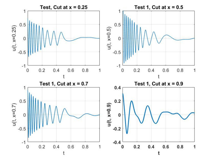
A delayed nonlinear wave equation with variable exponents of logarithmic type is discussed in this paper. In the presence of the logarithmic nonlinear source, we established a global existence result under sufficient conditions on the initial data only without imposing the Sobolev Logarithmic Inequality. After that, we established global results of exponential and polynomial types according to the range values of the exponents. At the end, we give a numerical study that supports our theoretical results.
- decay,
- nonlinearly damped,
- delay time,
- variable exponent
Citation: Mohammad Kafini, Maher Noor. Delayed wave equation with logarithmic variable-exponent nonlinearity[J]. Electronic Research Archive, 2023, 31(5): 2974-2993. doi: 10.3934/era.2023150

Related Papers:

Abstract

A delayed nonlinear wave equation with variable exponents of logarithmic type is discussed in this paper. In the presence of the logarithmic nonlinear source, we established a global existence result under sufficient conditions on the initial data only without imposing the Sobolev Logarithmic Inequality. After that, we established global results of exponential and polynomial types according to the range values of the exponents. At the end, we give a numerical study that supports our theoretical results.

References

[1]	H. A. Levine, Some additional remarks on the nonexistence of global solutions to nonlinear wave equations, SIAM J. Math. Anal., 5 (1974), 138–146. https://doi.org/10.1137/0505015 doi: 10.1137/0505015
[2]	M. Kopáčková, Remarks on bounded solutions of a semilinear dissipative hyperbolic equation, Commentat. Math. Univ. Carol., 30 (1989), 713–719.
[3]	E. Vitillaro, Global nonexistence theorems for a class of evolution equations with dissipation, Arch. Ration. Mech. Anal., 149 (1999), 155–182. https://doi.org/10.1007/s002050050171 doi: 10.1007/s002050050171
[4]	H. Levine, J. Serrin, Global nonexistence theorems for quasilinear evolution equations with dissipation, Arch. Ration. Mech. Anal., 137 (1997), 341–361. https://doi.org/10.1007/s002050050032 doi: 10.1007/s002050050032
[5]	Y. Wang, A global nonexistence theorem for viscoelastic equations with arbitrary positive initial energy, Appl. Math. Lett., 22 (2009), 1394–1400. https://doi.org/10.1016/j.aml.2009.01.052 doi: 10.1016/j.aml.2009.01.052
[6]	E. Zuazua, Exponential decay for the semilinear wave equation with locally distributed damping, Commun. Partial Differ. Equations, 15 (1990), 205–235. https://doi.org/10.1080/03605309908820684 doi: 10.1080/03605309908820684
[7]	Y. Ye, Global existence and blow-up of solutions for higher-order viscoelastic wave equation with a nonlinear source term, Nonlinear Anal. Theory Methods Appl., 112, (2015), 129–146. https://doi.org/10.1016/j.na.2014.09.001
[8]	S. Nicaise, C. Pignotti, Stability and instability results of the wave equation with a delay term in the boundary or internal feedbacks, SIAM J. Control Optim., 45 (2006), 1561–1585. https://doi.org/10.1137/060648891 doi: 10.1137/060648891
[9]	S. Nicaise, C. Pignotti, J. Valein, Exponential stability of the wave equation with boundary time-varying delay, Discrete Contin. Dyn. Syst. - Ser. S, 4 (2011), 693–722. https://doi.org/10.3934/dcdss.2011.4.693 doi: 10.3934/dcdss.2011.4.693
[10]	S. Nicaise, C. Pignotti, Stabilization of the wave equation with boundary or internal distributed delay, Differ. Integr. Equations, 2008 (2008), 935–958. https://doi.org/10.57262/die/1356038593 doi: 10.57262/die/1356038593
[11]	M. Kafini, S. A. Messaoudi, S. Nicaise, A blow-up result in a nonlinear abstract evolution system with delay, Nonlinear Differ. Equations Appl., 23 (2016), 1–14. https://doi.org/10.1007/s00030-016-0354-5 doi: 10.1007/s00030-016-0354-5
[12]	R. Aboulaich, D. Meskine, A. Souissi, New diffusion models in image processing, Comput. Math. Appl., 56 (2008), 874–882. https://doi.org/10.1016/j.camwa.2008.01.017 doi: 10.1016/j.camwa.2008.01.017
[13]	S. Lian, W. Gao, C. Cao, H. Yuan, Study of the solutions to a model porous medium equation with variable exponent of nonlinearity, J. Math. Anal. Appl., 342 (2008), 27–38. https://doi.org/10.1016/j.jmaa.2007.11.046 doi: 10.1016/j.jmaa.2007.11.046
[14]	Y. Chen, S. Levine, M. Rao, Variable exponent, linear growth functionals in image restoration, SIAM J. Appl. Math., 66 (2006), 1383–1406. https://doi.org/10.1137/050624522 doi: 10.1137/050624522
[15]	K. Ahmad, K. Bibi, New function solutions of ablowitz-kaup-newell-segur water wave equation via power index method, J. Funct. Spaces, 2022 (2022), 9405644.
[16]	A. M. Alghamdi, S. Gala, M. A. Ragusa, Global regularity for the 3d micropolar fluid flows, Filomat, 36 (2022), 1967–1970. https://doi.org/10.2298/FIL2206967A doi: 10.2298/FIL2206967A
[17]	H. Yüksekkaya, E. Piskin, Blow-up and decay of solutions for a delayed timoshenko equation with variable-exponents, Miskolc Math. Notes, 23 (2022), 1001–1022. https://doi.org/10.18514/MMN.2022.3890 doi: 10.18514/MMN.2022.3890
[18]	S. Antontsev, Wave equation with p (x, t)-laplacian and damping term: blow-up of solutions, C.R. Mec., 339 (2011), 751–755. https://doi.org/10.1016/j.crme.2011.09.001 doi: 10.1016/j.crme.2011.09.001
[19]	S. Antontsev, Wave equation with p (x, t)-laplacian and damping term: existence and blow-up, Differ. Equations Appl., 3 (2011), 503–525. https://doi.org/10.7153/dea-03-32 doi: 10.7153/dea-03-32
[20]	B. Guo, W. Gao, Blow-up of solutions to quasilinear hyperbolic equations with p (x, t)-laplacian and positive initial energy, C.R. Mec., 342 (2014), 513–519. https://doi.org/10.1016/j.crme.2014.06.001 doi: 10.1016/j.crme.2014.06.001
[21]	S. Antontsev, S. Shmarev, Evolution PDEs with Nonstandard Growth Conditions, Atlantis Press, Paris, France, 2015.
[22]	V. Galaktionov, S. Pohozaev, Blow-up and critical exponents for nonlinear hyperbolic equations, Nonlinear Anal. Theory Methods Appl., 53 (2003), 453–466. https://doi.org/10.1016/S0362-546X(02)00311-5 doi: 10.1016/S0362-546X(02)00311-5
[23]	S. H. Park, Blowup for nonlinearly damped viscoelastic equations with logarithmic source and delay terms, Adv. Differ. Equations, 2021 (2021), 1–14. https://doi.org/10.1186/s13662-020-03162-2 doi: 10.1186/s13662-020-03162-2
[24]	T. Yu, H. Yang, Initial boundary value problem for a class of strongly damped nonlinear wave equation, J. Harbin Eng. Univ., 25 (2004), 254–256. https://doi.org/10.1057/palgrave.jphp.3190034 doi: 10.1057/palgrave.jphp.3190034
[25]	T. G. Ha, S. H. Park, Blow-up phenomena for a viscoelastic wave equation with strong damping and logarithmic nonlinearity, Adv. Differ. Equations, 2020 (2020), 1–17. https://doi.org/10.1186/s13662-019-2438-0 doi: 10.1186/s13662-019-2438-0
[26]	L. Ma, Z. B. Fang, Energy decay estimates and infinite blow-up phenomena for a strongly damped semilinear wave equation with logarithmic nonlinear source, Math. Methods Appl. Sci., 41 (2018), 2639–2653. https://doi.org/10.1002/mma.4766 doi: 10.1002/mma.4766
[27]	S. H. Park, Global nonexistence for logarithmic wave equations with nonlinear damping and distributed delay terms, Nonlinear Anal. Real World Appl., 68 (2022), 103691. https://doi.org/10.1016/j.nonrwa.2022.103691 doi: 10.1016/j.nonrwa.2022.103691
[28]	M. Kafini, S. Messaoudi, Local existence and blow up of solutions to a logarithmic nonlinear wave equation with delay, Appl. Anal., 99 (2020), 530–547. https://doi.org/10.1080/00036811.2018.1504029 doi: 10.1080/00036811.2018.1504029
[29]	M. Kafini, S. Messaoudi, On the decay and global nonexistence of solutions to a damped wave equation with variable-exponent nonlinearity and delay, in Annales Polonici Mathematici, Instytut Matematyczny Polskiej Akademii Nauk, 122 (2019), 49–70.
[30]	B. Feng, Global well-posedness and stability for a viscoelastic plate equation with a time delay, Math. Probl. Eng., 2015 (2015), 585021.
[31]	V. Komornik, V. Gattulli, Exact controllability and stabilization. the multiplier method, SIAM Rev., 39 (1997), 351–351.

Reader Comments

Your name:*

Email:*
© 2023 the Author(s), licensee AIMS Press. This is an open access article distributed under the terms of the Creative Commons Attribution License (http://creativecommons.org/licenses/by/4.0)