Age and geographic dependence of Zika virus infection during the outbreak on Yap island, 2007

A. Endo; H. Nishiura; A. Endo; H. Nishiura

doi:10.3934/mbe.2020228

Mathematical Biosciences and Engineering

2020, Volume 17, Issue 4: 4115-4126. doi: 10.3934/mbe.2020228

Previous Article Next Article

Research article Special Issues

Age and geographic dependence of Zika virus infection during the outbreak on Yap island, 2007

A. Endo ^1,2,
H. Nishiura ^{1
,
,}

1.
Graduate School of Medicine, Hokkaido University, Kita 15 Jo Nishi 7 Chome, Kita-ku, Sapporo 060-8638, Japan
2.
Department of Infectious Disease Epidemiology, London School of Hygiene and Tropical Medicine, Keppel Street, Bloomsbury, London WC1E 7HT, United Kingdom

Received: 09 January 2020 Accepted: 06 May 2020 Published: 09 June 2020

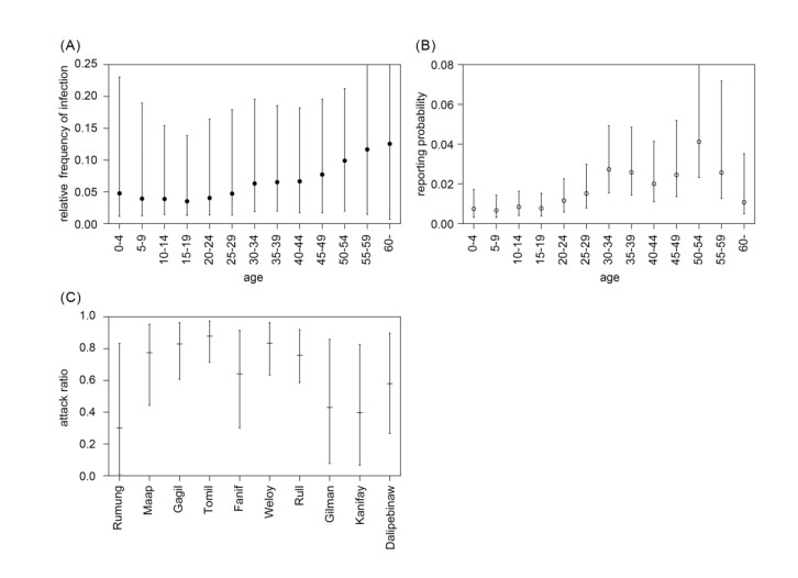
Intensive surveillance of Zika virus infection conducted on Yap Island has provided crucial information on the epidemiological characteristics of the virus, but the rate of infection and medical attendance stratified by age and geographical location of the epidemic have yet to be fully clarified. In the present study, we reanalyzed surveillance data reported in a previous study. Likelihood-based Bayesian inference was used to gauge the age and geographically dependent force of infection and age-dependent reporting rate, with unobservable variables imputed by the data augmentation method. The inferred age-dependent component of the force of infection was suggested to be up to 3-4 times higher among older adults than among children. The age-dependent reporting rate ranged from 0.7% (5-9 years old) to 3.3% (50-54 years old). The proportion of serologically confirmed cases among total probable or confirmed cases was estimated to be 44.9%. The cumulative incidence of infection varied by municipality: Median values were over 80% in multiple locations (Gagil, Tomil, and Weloy), but relatively low values (below 50%) were derived in other locations. However, the possibility of a comparably high incidence of infection was not excluded even in municipalities with the lowest estimates. The results suggested a high degree of heterogeneity in the Yap epidemic. The force of infection and reporting rate were higher among older age groups, and this discrepancy implied that the demographic patterns were remarkably different between all infected and medically attended individuals. A higher reporting rate may have reflected more severe clinical presentation among adults. The symptomatic ratio in dengue cases is known to correlate with age, and our findings presumably indicate a similar tendency in Zika virus disease.

Keywords:

Citation: A. Endo, H. Nishiura. Age and geographic dependence of Zika virus infection during the outbreak on Yap island, 2007[J]. Mathematical Biosciences and Engineering, 2020, 17(4): 4115-4126. doi: 10.3934/mbe.2020228

Related Papers:

[1]	Christian Winkel, Simon Neumann, Christina Surulescu, Peter Scheurich . A minimal mathematical model for the initial molecular interactions of death receptor signalling. Mathematical Biosciences and Engineering, 2012, 9(3): 663-683. doi: 10.3934/mbe.2012.9.663
[2]	Hong Yuan, Jing Huang, Jin Li . Protein-ligand binding affinity prediction model based on graph attention network. Mathematical Biosciences and Engineering, 2021, 18(6): 9148-9162. doi: 10.3934/mbe.2021451
[3]	Yuewu Liu, Mengfang Zeng, Shengyong Liu, Chun Li . Dynamics analysis of building block synthesis reactions for virus assembly in vitro. Mathematical Biosciences and Engineering, 2023, 20(2): 4082-4102. doi: 10.3934/mbe.2023191
[4]	Ronald Lai, Trachette L. Jackson . A Mathematical Model of Receptor-Mediated Apoptosis: Dying to Know Why FasL is a Trimer. Mathematical Biosciences and Engineering, 2004, 1(2): 325-338. doi: 10.3934/mbe.2004.1.325
[5]	Feng Rao, Carlos Castillo-Chavez, Yun Kang . Dynamics of a stochastic delayed Harrison-type predation model: Effects of delay and stochastic components. Mathematical Biosciences and Engineering, 2018, 15(6): 1401-1423. doi: 10.3934/mbe.2018064
[6]	Max-Olivier Hongler, Roger Filliger, Olivier Gallay . Local versus nonlocal barycentric interactions in 1D agent dynamics. Mathematical Biosciences and Engineering, 2014, 11(2): 303-315. doi: 10.3934/mbe.2014.11.303
[7]	Yutong Man, Guangming Liu, Kuo Yang, Xuezhong Zhou . SNFM: A semi-supervised NMF algorithm for detecting biological functional modules. Mathematical Biosciences and Engineering, 2019, 16(4): 1933-1948. doi: 10.3934/mbe.2019094
[8]	O. E. Adebayo, S. Urcun, G. Rolin, S. P. A. Bordas, D. Trucu, R. Eftimie . Mathematical investigation of normal and abnormal wound healing dynamics: local and non-local models. Mathematical Biosciences and Engineering, 2023, 20(9): 17446-17498. doi: 10.3934/mbe.2023776
[9]	Zhenzhen Zheng, Ching-Shan Chou, Tau-Mu Yi, Qing Nie . Mathematical analysis of steady-state solutions in compartment and continuum models of cell polarization. Mathematical Biosciences and Engineering, 2011, 8(4): 1135-1168. doi: 10.3934/mbe.2011.8.1135
[10]	Linlu Song, Shangbo Ning, Jinxuan Hou, Yunjie Zhao . Performance of protein-ligand docking with CDK4/6 inhibitors: a case study. Mathematical Biosciences and Engineering, 2021, 18(1): 456-470. doi: 10.3934/mbe.2021025

Abstract

1. Introduction

Ligands, are biochemical modifiers of macromolecular structure and can impact biological function. These can be co-factors (iron, cobalt, copper, zinc), co-enzymes such as Nicotinamide- and Flavin- Adenine Dinucleotides (NAD, FAD) and full-length molecules with short binding sites ^[1,2]. Ligands, unlike substrates/co-substrates are either reversibly altered or not at all. The biochemical role of ligands, in vivo, is complex and can influence both, enzyme-mediated substrate catalysis and non-enzymatic association and dissociation interactions. Whilst, the interaction with competitive inhibitors, co-factors or co-enzymes involves definitive and direct modifications to the active site residues, the effect of a ligand can be allosteric and indirect ^[3,4,5]. The latter involves both long-distance conformational changes and non-covalent interactions (hydrogen, Van der Waals, hydrophobic, electrostatic) ^{[6,7,8,9,10,11]}. Empirical data suggests that the binding affinity or the strength-of-association of a macromolecule for its ligand is a critical determinant of function ^{[7,8,9,10,11]}. For example, 2, 3-Bisphophoglycerate is a potent modifier of Hemoglobin function and does so by shifting the oxygen-dissociation curve to the right. In its absence Hemoglobin retains high affinity for molecular oxygen (left-shift of the oxygen dissociation curve), an undesirable effect on its role as a transporter ^[10,11]. Similarly, Ascorbic acid maintains iron in its reduced state in the gastrointestinal tract and as part of the active site of non-haem iron (Ⅱ)- and 2-oxoglutarate-dependent dioxygenases ^[12,13]. Deficiency of Ascorbic acid is implicated in tardy iron absorption in the ileum as well as a range of collagen disorders such as scurvy (Prolyl- and Lysyl-hydroxylases) ^[14,15]. Conversely, proteins which are modified such as those that may originate from missense or amino acid substitutions and are secondary to genomic variants such as single nucleotide polymorphisms (SNPs) and insertions-deletions (indels), will also result in several clinical outcomes ^[16,17]. Here, too, enzyme catalysis is directly affected if these are present at the active site or is impacted indirectly (folding, stability, complex formation) when present elsewhere ^[16,17,18].

There is a large volume of literature which describes macromolecules in terms of either residues (amino acids, nucleotides) interacting or an all atom-based interaction matrix. The proponent of the 2D approach is the Gaussian network model (GNM), while the Anisotropic network model (ANM) is representative of the 3D approach ^{[19,20,21,22]}. The fundamental premise of both these approaches is the elastic network model (ENM) ^[19]. Here, an atom or residue is modeled as an elastic mass and the interaction between a pair of atoms/residues is dependent on the selection of a pre-determined cut-off distance ^[22]. The force constant, although, not a parameter by definition, has also been studied and shows good correlation with B-factor data ^[23]. A major application of these studies is normal mode analysis (NMA), which has been used to glean valuable insights into the structural dynamics of the investigated macromolecule and into B-factor distribution ^[23,24]. Despite this success, there are significant limitations of this approach, including inadequate descriptors for the type of interactions computed by the Hessian matrix and data points that are dependent on a preselected cut-off distance (5–10 Ang, GNM; 10–15 Ang, ANM) ^[20,22,25]. Parameter-free versions of the ENM (pfENM), GNM (pfGNM) and ANM (pfANM), to resolve the latter, have been described and compared to establish B-factor distribution (isotropic, anisotropic) ^[25]. Additionally, many of these studies have focused on inferring biophysical characteristics such as cross-correlational fluctuations and mean square displacements. From a functional standpoint, however, it is not clear whether these data can be utilized to derive/study parameters such as the Michaelis-Menten constant (Km) or the association/dissociation (Ka/Kd). Since, these depend on the presence of an organic or inorganic modifier, i.e., ligand/substrate/co-factor/co-substrate, in addition to the modeled macromolecule, its exclusion is another major lacuna of these studies.

Despite the availability of clinical, empirical, analytical and computational data, a mathematically rigorous explanation for the heterogeneity in biochemical function, for a ligand-macromolecular complex, is missing. The work presented models a ligand and macromolecule as a homo- or hetero-dimer and subsumes a finite and equal number of atoms/residues per monomer. The pairwise interactions of the resulting square matrix will be chosen randomly from a standard uniform distribution. The resulting eigenvalues will be analyzed and modeled in accordance with known literature on biochemical reactions to generate biologically viable and usable dissociation constants. The theoretical results will be complemented by numerical studies where applicable. Additionally, and through various theorems, lemmas and corollaries, a schema to partition ligands into high- and low-affinity variants will also be discussed. The suitability of the transition-state dissociation constants as a model for ligand-macromolecular interactions will be inferentially assessed by analyzing the clinical outcomes of amino acid substitutions of selected enzyme homodimers. The relevance of the model to biochemical function will be discussed by examining the ligand-macromolecular complex for known ligands of non-haem iron (Ⅱ)- and 2-oxoglutarate-dependent dioxygenases (Fe2OG) and the major histocompatibility complex (Ⅰ) (MHC1).

The general outline of the manuscript includes an initial section where the system to be modeled, rationale for this study, and formal definitions are introduced (Section 2). The model is analyzed, formulated and presented as theorems, lemmas and corollaries (Section 3). This section also includes a numerical study to demonstrate and validate the theoretical assertions made. The biological relevance of these findings are discussed with an analysis of clinical outcomes of enzyme sequence variants and case studies of enzyme- and non-enzymatic complex formation (Section 4). A brief conclusion that summarizes the presented study, limitations and future directions is included at the end of the manuscript (Section 5). Details of all proofs are included after the conclusions (Section 6).

2. Model description and definitions

Consider the generic interaction between macromolecule $\left(c\right)$ and ligand $\left(\mu \right)$ ,

$\begin{array}{cc}c\mu \begin{array}{c}\stackrel{{r}_{f}}{\to }\\ \underset{{r}_{b}}{\leftarrow }\end{array}c+\mu & RXN\left(1\right)\end{array}$

We can represent this interaction/reaction, at a steady state, with the rate equations ^[26],

${R}_{d}\left(c\mu \right) = {r}_{f}.{\left[c\mu \right]}^{{L}_{c\mu }\ge 0}$

(1)

${{R}_{a}\left(c\mu \right) = {r}_{b}.\left[c\right]}^{{L}_{c}\ge 0}{\left[\mu \right]}^{{L}_{\mu }\ge 0}$

(2)

At steady state,

${R}_{d}\left(c\mu \right) = {R}_{a}\left(c\mu \right)$

(3)

$\Rightarrow \frac{{r}_{f}}{{r}_{b}} = \frac{{\left[c\right]}^{{L}_{c}\ge 0}.{\left[\mu \right]}^{{L}_{\mu }\ge 0}}{{\left[c\mu \right]}^{{L}_{c\mu }\ge 0}}$

(4)

$\frac{{r}_{f}}{{r}_{b}} = Kd\left(c\mu \right)$

(5)

Here,

$c: = Macromolecule$

$\mu : = Ligand$

$\left[.\right]: = Molar\;concentration\;of\;reactant\;in\;standard\;form\;\left(M\right)$

${R}_{a}\left(c\mu \right): = Rate\;of\;association\;of\;complex\;\left(M{s}^{-1}\right)$

${R}_{d}\left(c\mu \right): = Rate\;of\;dissociation\;of\;complex\;\left(M{s}^{-1}\right)$

${r}_{f}: = Rate\;constants\;of\;forward\;reaction\;\left({s}^{-1}\right)$

${r}_{b}: = Rate\;constants\;of\;reverse\;reaction\left({M}^{-1}{s}^{-1}\right)$

$L: = Stoichiometry\;of\;reactant\left(s\right)$

$Kd\left(c\mu \right): = Dissociation\;constant\;for\;ligand-macromolecular\;complex\left(M\right)$

It is clear that a ligand-macromolecular complex may exist in one of three distinct states. These include: a) perfect association, b) perfect dissociation and c) an intermediate- or transition-state; and can be represented in terms of the dissociation constant,

Case (1) $Perfect\;association$ Def. (1)

$\frac{1}{{r}_{b}}\to \infty ;{r}_{f}\to 0$

(6, 7)

$\Rightarrow Kd\left(c\mu \right)\approx 0$

(8)

Case (2) $Perfect\;disassociation$ Def. (2)

${r}_{f} > > > {r}_{b}$

(9)

$\Rightarrow Kd\left(c\mu \right)\ge 1$

(10)

Case (3) $Transient-state\;disassociation\;constant$ Def. (3)

${r}_{f}\lessgtr {r}_{b}$

(11)

$\Rightarrow Kd\left(c\mu \right)\in \mathbb{R}\cap \left(\mathrm{0, 1}\right)$

(12)

Consider an atom/residue-based representation (amino acids/nucleotides) of a generic set of monomeric macromolecules, ${\boldsymbol{\mathcal{C}}} = \{protein, DNA, RNA\}$ , with $z = \mathrm{1, 2}, \dots ., Z$ components each with $i$ -indexed ( $i = \mathrm{1, 2}, \dots ., I$ ) c-atoms/residues,

$\begin{array}{cc}{{\bf c}\equiv {{{\mathcal{C}}}}_{z}\in {\boldsymbol{\mathcal{C}}}|{\bf c} = \left[{c}_{1}{c}_{2}\dots .{c}_{i = I}\right]}^{T}, I\in \mathbb{N}& \end{array}$

(13)

The analogous model of a monomer ligand, ${\boldsymbol{\mathcal{L}}} = \{small\;molecule, peptide, oligonucleotide\}$ , with $j$ -indexed $(j = \mathrm{1, 2}, \dots , J)$ $\mu$ -atoms/residues is,

$\boldsymbol{\mu }\in {\boldsymbol{\mathcal{L}}}|{\bf{ \pmb{\mathsf{ μ}} }} = \left[{\mu }_{1}{\mu }_{2}\dots .{\mu }_{j = J}\right], J\in \mathbb{N}$

(14)

It is also assumed that the ligand-macromolecular complex is a homo- or hetero-dimer with an equal number of atoms/residues $\left(I = J\right)$ per monomer. The interaction matrix is,

$\begin{array}{rr}\left\langle{\boldsymbol{c}|\boldsymbol{\mu }}\right\rangle = {\left[{c}_{1}{c}_{2}..{c}_{i = I}\right]}^{T}\times \left[{\mu }_{1}{\mu }_{2}..{\mu }_{j = J}\right] = {{\boldsymbol{\mathcal{C}}}}_{\boldsymbol{z}\boldsymbol{\mu }} = \left({{c}_{i}\mu }_{j}\right)\subset {\mathbb{R}}^{I\times J}& \end{array}$

(15)

The numerical values of this matrix are chosen randomly from the standard uniform distribution,

$\begin{array}{rr}{{\boldsymbol{\mathcal{C}}}}_{z\mu } = \left({{c}_{i}\mu }_{j}\right)\in {\mathcal{U}}_{\left[\mathrm{0, 1}\right]}& \end{array}$

(16)

The rationale for this choice is that each pairwise interaction is subsumed to be a function of an arbitrary number of non-bonded interactions (long- and short-range) and is therefore, unique. Clearly, this implies the existence of $\left\{I, J\right\}$ -linear independent vectors,

$\begin{array}{cc}rank\left({{\boldsymbol{\mathcal{C}}}}_{z\mu }\right) = \left\{I, J\right\}& \end{array}$

(17)

Since ${{\boldsymbol{\mathcal{C}}}}_{\boldsymbol{z}\boldsymbol{\mu }}$ is diagonalizable there exists a diagonal matrix, $\mathit{\boldsymbol{\mathcal{K}}{\boldsymbol{\mathcal{C}}}}_{z\mu }$ ,

$\mathit{\boldsymbol{\mathcal{K}}{\boldsymbol{\mathcal{C}}}}_{z\mu } = {\boldsymbol{X}}^{-1}{{\boldsymbol{\mathcal{C}}}}_{z\mu }\boldsymbol{X}$

(18)

${z}_{i = j} = z\in diag\left(\mathit{\boldsymbol{\mathcal{K}}{\boldsymbol{\mathcal{C}}}}_{z\mu }\right)\subset \mathbb{C}$

(19)

${{\boldsymbol{\mathcal{C}}}}_{\boldsymbol{z}\boldsymbol{\mu }}$ , is non-symmetric the computed eigenvalues of the modeled ligand-macromolecular interaction matrix can have positive and negative real parts,

$\left\{{\alpha }_{ij} = Re\left(z\right)\in \boldsymbol{K}\boldsymbol{d}\left({{\boldsymbol{\mathcal{C}}}}_{\boldsymbol{z}\boldsymbol{\mu }}\right)\subset \mathbb{R}|i = j, z\in \mathbb{C}\right\}$

(20)

$\left\{{\alpha }_{ij} = Re\left(z\right)\in \boldsymbol{K}\boldsymbol{d}\left({{\boldsymbol{\mathcal{C}}}}_{\boldsymbol{z}\boldsymbol{\mu }}\right)\subset \mathbb{R}|i = j, z\in \mathbb{C}\right\}$

(20.1)

A further subdivision can be made in accordance with established literature,

$\left\{{\alpha }_{ij} = Re\left(z\right)\in \boldsymbol{K}\boldsymbol{d}\left({{\boldsymbol{\mathcal{C}}}}_{\boldsymbol{z}\boldsymbol{\mu }}\right)\subset \mathbb{R}|i = j, z\in \mathbb{C}\right\} {\omega }_{\infty } = Kd\left(c\mu \right)\ge 1$

(21)

$Perfect\;association\equiv Reverse \;\; {\omega }_{0} = Kd\left(c\mu \right) = 0$

(22)

This selection generates the set,

$\omega = {\alpha }_{ij}\in \boldsymbol{K}\boldsymbol{d}\left({{\boldsymbol{\mathcal{C}}}}_{\boldsymbol{z}\boldsymbol{\mu }}\right)\subset \mathbb{R}\cap \left(\mathrm{0, 1}\right)$

(23)

$\omega \in \boldsymbol{K}\boldsymbol{d}\left(\boldsymbol{c}\boldsymbol{\mu }\right)\;\;\;\;\;\;\;\;\;\;\;\;\;\;\;\;\;\;\;\;\;\;\;\;\;\;\;\;\;Def.\; {\mathit{(4)}}$

$\#\boldsymbol{K}\boldsymbol{d}\left(\boldsymbol{c}\boldsymbol{\mu }\right) = A$

(23.1)

We can combine these to get a preliminary definition of the transition-state disassociation constants. These are the strictly positive real part of all complex eigenvalues that characterize a ligand-macromolecular complex with an equal number of atoms/residues per monomer and belong to the open interval (0, 1),

$\left\{\omega = \mathcal{R}\mathrm{e}\left(\mathrm{z}\right)\in \boldsymbol{K}\boldsymbol{d}\left(\boldsymbol{c}\boldsymbol{\mu }\right)\subset \boldsymbol{K}\boldsymbol{d}\left({{\boldsymbol{\mathcal{C}}}}_{\boldsymbol{z}\boldsymbol{\mu }}\right)\subset \mathbb{R}\cap \left(\mathrm{0, 1}\right)|z\in \mathbb{C}\right\}$

(

$Def. \; {\mathit{(5a)}}$ )

3. Results

3.1. Mathematical analysis of transition-state dissociation constants of the modeled ligand-macromolecular complex

Whilst, the states of perfect association and dissociation are key determinants of whether a reaction will occur or not, the transition-state dissociation constants may offer insights into the origins of threshold values, feedback mechanisms and other regulatory checkpoints. However, in order to ascribe biological relevance to these findings we must establish various bounds which can then be utilized to assess and thence assay the function of a ligand-macromolecular complex.

Theorem 1 (T1): The linear map between the transition-state dissociation constants and the eigenvalues that characterize the interactions of the homo- or hetero-dimer form of the modeled ligand-macromolecular complex is the injection,

$g:\omega \in \boldsymbol{K}\boldsymbol{d}\left(\boldsymbol{c}\boldsymbol{\mu }\right)\mapsto \boldsymbol{K}\boldsymbol{d}\left({{\boldsymbol{\mathcal{C}}}}_{\boldsymbol{z}\boldsymbol{\mu }}\right)$

(24)

Theorem 2 (T2): The transition-state dissociation constants that characterize the interactions of the homo- or hetero-dimer form of the modeled ligand-macromolecular complex is a monotonic and non-increasing sequence,

$\begin{array}{cc}{\left\{{\omega }_{a}\right\}}_{a\le a+1}|& \omega \in \boldsymbol{K}\boldsymbol{d}\left(\boldsymbol{c}\boldsymbol{\mu }\right)\end{array}$

(25)

Theorem 3 (T3): The transition-state dissociation constants that characterize the interactions of the homo- or hetero-dimer form of the modeled ligand-macromolecule complex are monotonic, bounded and therefore, convergent,

$\begin{array}{cc}\underset{a\to \infty }{\mathrm{lim}}{\left\{{\omega }_{a}\right\}}_{a\le a+1} = \left\{\mathrm{0, 1}\right\}|& \omega \in \boldsymbol{K}\boldsymbol{d}\left(\boldsymbol{c}\boldsymbol{\mu }\right)\end{array}$

(26)

Corollary 1 (C1): The transition-state dissociation constants that characterize the interactions of the homo- or hetero-dimer form of the modeled ligand-macromolecule complex is a sequence with defined greatest-lower and least-upper -bounds,

$inf{\left\{{\omega }_{a}\right\}}_{a\le a+1} < {\left\{{\omega }_{a}\right\}}_{a\le a+1} < sup{\left\{{\omega }_{a}\right\}}_{a\le a+1}$

(27)

Corollary 2 (C2; without proof): The cardinality of the set of transition-state dissociation constants that characterize the interactions of the homo- or hetero-dimer form of the modeled ligand-macromolecule complex is finite,

$\begin{array}{c}\#\boldsymbol{K}\boldsymbol{d}\left(\boldsymbol{c}\boldsymbol{\mu }\right) = A < \#\boldsymbol{K}\boldsymbol{d}\left({{\boldsymbol{\mathcal{C}}}}_{\boldsymbol{z}\boldsymbol{\mu }}\right) = \left\{I, J\right\}\end{array}$

(28)

Using T1–T3 and C1, C2 we can refine our definition of the transition-state dissociation constants for the modeled ligand-macromolecular complex,

$\begin{array}{cc}{\left\{{\omega }_{a}\right\}}_{a\le a+1}|& \omega \in \boldsymbol{K}\boldsymbol{d}\left(\boldsymbol{c}\boldsymbol{\mu }\right)\end{array};a = \mathrm{1, 2}\dots A$

(

$Def. \; {\mathit{(5b)}}$ )

where,

$\omega = \mathcal{R}\mathrm{e}\left(\mathrm{z}\right)\in \boldsymbol{K}\boldsymbol{d}\left({{\boldsymbol{\mathcal{C}}}}_{\boldsymbol{z}\boldsymbol{\mu }}\right)\subset \mathbb{R}\cap \left(\mathrm{0, 1}\right)|z\in \mathbb{C}$

3.2. Annotation of a ligand on the basis of the transition-state dissociation constants of the modeled ligand-macromolecular complex

It is clear from the above results that the eigenvalue-based transition-state dissociation constants are continuous and can potentially model the multiplicity of intermediate- or transient-states that a ligand-macromolecular complex may adopt. It should therefore, be possible to partition the transition-state dissociation constants into functionally distinct subsets and will be characteristic for a specific ligand-macromolecular complex.

Theorem 4 (T4): The transition-state dissociation constants that characterize the interactions of the homo- or hetero-dimer form of the modeled ligand-macromolecule complex is a proper subset of the complete set of the real part of all complex eigenvalues that comprise the interaction matrix,

$\boldsymbol{K}\boldsymbol{d}\left(\boldsymbol{c}\boldsymbol{\mu }\right)\subset \boldsymbol{K}\boldsymbol{d}\left({{\boldsymbol{\mathcal{C}}}}_{\boldsymbol{z}\boldsymbol{\mu }}\right)$

(29)

Corollary 3 (C3): The distribution of the transition-state dissociation constants that characterize the interactions of the homo- or hetero-dimer form of the modeled ligand-macromolecule complex will result in a schema by which we can annotate the ligand as a high $\left({\mu }_{high}\right)$ - or low $\left({\mu }_{low}\right)$ -affinity variant,

$\mu = \left\{{\mu }_{high}, {\mu }_{low}\right\}$

(30)

3.3. Modeling the transition-state dissociation constants of higher-order ligand-macromolecular complexes

Biologically relevant macromolecular complexes are characterized by heterogeneity and high-order $\left(Z\ge 2\right)$ . This multimer-form of a macromolecule is formed around a primary molecule and its interactions. These may be protein-protein, DNA/RNA-protein or DNA-RNA-protein.

The multimer-form of ligand-macromolecular complex is easily modeled using the mathematical framework defined earlier. Here, the ligand-macromolecular complex is considered as a set of interacting monomers and the binding to a ligand occurs via a single unique monomer,

$\left\{{{{\mathcal{C}}}}_{z}\in {\boldsymbol{\mathcal{C}}}|{{{\mathcal{C}}}}_{1} = {{{\mathcal{C}}}}_{2}\dots = {{{\mathcal{C}}}}_{z = Z}|Z\ge 2\right\}$

(

$Def. \; {\mathit{(6a)}}$ )

where,

${{{\mathcal{C}}}}_{z}\equiv {{{\mathcal{C}}}}_{z\mu }\equiv \mu {{{\mathcal{C}}}}_{z}$

(

$Def. \; {\mathit{(6b)}}$ )

Here,

$\mu : = Ligand$

${{{\mathcal{C}}}}_{z}: = Unique\;monomer\;of\;a\;macromolecule\;that\;associates\;with\;a\;ligand$

$\mu {{{\mathcal{C}}}}_{z}: = Ligand-macromolecular\;complex$

On the basis of these definitions we can re-index the remaining monomers, i.e., after excluding the unique monomer that binds to the ligand,

$\left\{{{{\mathcal{C}}}}_{y}\in \widetilde {{\boldsymbol{\mathcal{C}}}} = {\boldsymbol{\mathcal{C}}}\backslash \left\{{{{\mathcal{C}}}}_{z}\right\}|y = \mathrm{1, 2}\dots Y;Y = Z-1\right\}$

(

$Def. \; {\mathit{(7)}}$ )

We now derive an expression for the multimer (higher-order)-form of a ligand-macromolecular complex.

Theorem 5 (T5): The multimer-form of a ligand-macromolecular complex comprising identical monomer units and with an arbitrary unit associating with a ligand is,

$\begin{array}{rr}{\prod }_{y = 1}^{y = Y}{{{\mathcal{C}}}}_{z}.{\mathcal{C}}_{y} = {\mathcal{C}}_{z}.{\mathcal{C}}_{Y}^{y}|y = \mathrm{1, 2}\dots Y;Y = Z-1;Z\ge 2;z = \mathrm{1, 2}\dots Z& \end{array}$

(31)

Rewriting, this result in terms of the definition of the multimer form of a ligand-macromolecular complex,

$\begin{array}{cc}{\mathcal{C}}_{z}.{\mathcal{C}}^{Y}\equiv \mu {\mathcal{C}}_{z}.{\mathcal{C}}^{Y}& \end{array}$

(

$Def. \; {\mathit{(8)}}$ )

Theorem 6 (T6): The linear map between the transition-state dissociation constants that characterize the interactions of the monomer- and multimer-forms of a ligand-macromolecular complex is a bijection,

$\begin{array}{cc}{h}^{-1}\circ h:\omega \in \boldsymbol{K}\boldsymbol{d}\left(\boldsymbol{c}\boldsymbol{\mu }\right)\leftrightarrow u\in \boldsymbol{K}\boldsymbol{d}\left(\mu \boldsymbol{\mathcal{C}}_{z}\right)& \end{array}$

(32)

Theorem 7 (T7): The linear map between the transition-state dissociation constants and the eigenvalues that characterize the multimer-form of a ligand-macromolecular complex is a composition and an injection,

$\begin{array}{cc}g\circ {h}^{-1}\circ h:u\in \boldsymbol{K}\boldsymbol{d}\left(\mu \boldsymbol{\mathcal{C}}_{z}.{\mathcal{C}}^{Y}\right)\mapsto \boldsymbol{K}\boldsymbol{d}\left(\boldsymbol{\mathcal{C}}_{\boldsymbol{z}\boldsymbol{\mu }}\right)& \end{array}$

(33)

3.4. Numerical studies to establish biological relevance of the transition-state dissociation constants

The aforementioned theoretical results establish the mathematical rigor behind the definition and development of the transition-state dissociation constants as a model for ligand-macromolecular interactions (T1–T7, C1–C3). These assertions are complemented and numerically validated in R-4.1.2. Here, the R-packages, "ConvergenceConcepts" and "pracma" are utilized to investigate and analyze the stochastic convergence of the eigenvalues generated by the interaction matrix of a ligand-macromolecular complex (Supplementary Text 1) ^[27]. The R-scripts to establish convergence along with data processing are developed in-house (Supplementary Text 2). The stepwise algorithm to compute and numerically validate the transition-state dissociation constants is presented (Figure 1).

Figure 1. Numerical studies of ligand-macromolecular interactions as eigenvalue-based transition-state dissociation constants.

DownLoad: Full-Size Img PowerPoint

Step 1: A ligand and macromolecule with an equal number of atoms/residues ( $n = 25$ ) is chosen. Whilst, the complex can be modeled as a perfect homodimer, imperfect forms such as alternatively spliced isoenzymes are prevalent and commonly observed. Alternatively, the ligand can be modeled as a different macromolecule altogether.

Step 2: Populate the square interaction matrix with values randomly chosen from a uniform distribution, ${\mathcal{U}}_{\left[\mathrm{0, 1}\right]}$ . These will represent one of three potential states for each interacting pair of atoms/residues of the modeled ligand-macromolecular complex (association, complete disassembly, transition-state).

Step 3: Compute the complex eigenvalues of this matrix and extract the real part of each.

Step 4: Form a sequence of the subset comprising those values that are strictly positive and belong to the open interval $\left(\mathrm{0, 1}\right)$ .

Step 5: Establish the stochastic convergence in distribution and/or probability of the terms of this sequence to the expected upper (tsup)- and lower (tinf)-bounds, i.e., 0 and 1.

Step 5.1: Construct a sequence of random numbers, X, whose elements are uniquely mapped to the eigenvalue-based transition-state dissociation constants and represent intermediate- or transition-states of the modeled ligand-macromolecular complex,

$\left\{{X}_{a}\in \boldsymbol{X}\cap \boldsymbol{K}\boldsymbol{d}\left(\boldsymbol{c}\boldsymbol{\mu }\right)\subset \mathbb{R}\cap \left(\mathrm{0, 1}\right)|a = \mathrm{1, 2}\dots A\right\}$

(

$Def. \; {\mathit{(9)}}$ )

Here,

$A = \#\left(\boldsymbol{X}\cap \boldsymbol{K}\boldsymbol{d}\left(\boldsymbol{c}\boldsymbol{\mu }\right)\right)$

(34)

Step 5.2: Establish convergence of this set of random numbers. Here, weak convergence will suffice (distribution, probability),

$\underset{a\to \infty }{\mathrm{lim}}\left({X}_{a}\right)\to \left\{tinf, tsup\right\} = \left\{\mathrm{0, 1}\right\}$

(35)

The parameters to accomplish this numerically are,

$\begin{array}{r}nmax: = Number\;of\;values\;to\;analyse\\ M: = Number\;of\;paths\\ \varepsilon : = Threshold\;value\\ tinf: = Lower\;limit\;of\;interval\;to\;establish\;convergence\\ tsup: = Upper\;limit\;of\;interval\;to\;establish\;convergence\end{array}$

The values of these parameters for the numerically studied example are,

$nmax = A = 11$

(35.1)

$M = 500$

(35.2)

$\varepsilon = 0.01$

(35.3)

$tinf = 0$

(35.4)

$tsup = 1$

(35.5)

4. Discussion

The eigenvalue-based model of transition-state dissociation constants of a ligand-macromolecular complex asserts that there are several intermediate- or transition-states of a complex and that each of these has the potential to modify the biochemical process that the complex participates in.

4.1. Transition-state dissociation constants as a model of biochemical function for ligand-macromolecular complexes

Ligand-macromolecular complexes, in vivo, possess a finite and in most cases, an incomparable number of atoms/residues. The theoretical results establish definition(s), bounds and metrics to assess biochemical function for both, monomer (T1–T4, C1–C3)- and multimer (T5–T7)-forms. The numerical data suggests that the set of transition-state dissociation constants can be finite, converge and retain statistical relevance (Figure 1).

Proposition (P): The transition-state dissociation constants for the monomer ( $z = Z = 1$ )- and multimer ( $Z\ge 2$ )-forms of a ligand-macromolecular complex with a finite number of atoms/residues of each $\left(I, J\right)$ per monomer,

$\left\{u\in \boldsymbol{K}\boldsymbol{d}\left(\boldsymbol{\mu }\boldsymbol{\mathcal{C}}_{\boldsymbol{z}}.\boldsymbol{\mathcal{C}}^{\boldsymbol{Y}}\right)|{\mathcal{C}}_{z}\in \boldsymbol{\mathcal{C}}, \mu \in {\boldsymbol{\mathcal{L}}};z = \mathrm{1, 2}\dots Z;A = \left\{I, J\right\}\right\}$

(

$Def. \; {\mathit{(10)}}$ )

is the finite set,

$\boldsymbol{K}\boldsymbol{d}\left(\boldsymbol{\mu }\boldsymbol{\mathcal{C}}_{\boldsymbol{z}}.\boldsymbol{\mathcal{C}}^{\boldsymbol{Y}}\right)\subset \boldsymbol{K}\boldsymbol{d}\left(\boldsymbol{\mathcal{C}}_{\boldsymbol{z}\boldsymbol{\mu }}\right)$

Here,

$I = \#{\mathcal{C}}_{z}|{\mathcal{C}}_{z}\in \boldsymbol{\mathcal{C}}$

(36)

$J = \#\mu |\mu \in {\boldsymbol{\mathcal{L}}}$

(37)

where,

$\boldsymbol{K}\boldsymbol{d}\left(.\right): = Set\;of\;constrained\;eigenvalue-based\;transition-state\;dissociation\;constants$

$I: = Finite\;number\;of\;atoms\;or\;residues\;of\;macromolecule$

$J: = Finite\;number\;of\;atoms\;or\;residues\;of\;ligand$

${\mathcal{C}}_{\mu z}.{\mathcal{C}}^{Y}: = Multimer\;form\;of\;ligand-macromolecular\;complex$

Enzyme-mediated catalysis, or lack thereof, results in metabolic enzyme disorders and may be inherited (inborn errors of metabolism) or acquired ^[28]. In order to assess the biomedical relevance of modeling ligand-macromolecule interactions as transition-state dissociation constants, the clinical outcomes of amino acid substitutions of selected enzyme homo- or hetero-dimers are examined (). These outcomes, i.e., benign, likely benign, pathologic, likely pathologic, conflicting, uncertain significance, are defined in accordance with the prevalent nomenclature of the ClinVar database ^[16]. Here, the data annotated as "uncertain significance" are those sequence variants with a high likelihood ( $\approx 90–95\%$ ) of being "benign" or "pathogenic" ^[17]. This means they are likely to classified as "true positive", and if ignored will result in a "false negative". On the other hand, an outcome designated as with a "conflicting interpretation" is likely to be due to unresolved contradictory findings in the presence or absence of confounding factors. If we assume perfect contradiction, i.e., 50%, and couple this with the previous result, we get a $\approx 70–73\%$ possibility that the variant of interest is a "true positive". This means, that here too, if missed a "false negative" will result. The metric of choice is the Recall (R) percentage,

$R = \frac{TP}{TP+FN}\times 100$

(38)

$R: = Recall$

$\begin{array}{l} TP: = Known\;positives(benign, likelybenign,\\ pathogenic, likely\;pathogenic) \end{array}$

(

$Def. \; {\mathit{(12)}}$ )

$\begin{array}{l} FN: = Likely\;positives(conflicting\\ \;data, uncertain\;significance) \end{array}$

(

$Def. \; {\mathit{(13)}}$ )

Table 1. Analysis of clinical outcomes of amino acid substitutions of selected enzyme homo- and hetero-dimer forms present in ClinVar.

	Enzyme	EC	CV	SNP	M	Co	US	B	LB	P	LP	FN	TP	R (%)
1	Glucokinase	2.7.1.2	778	619	370	49	157	4	4	65	113	206	186	47.45
2	Pyruvate kinase	2.7.1.40	1239	629	209	14	135	7	7	30	20	149	64	30.05
3	Cathepsin A	3.4.16.x	1776	1270	501	20	382	26	23	26	34	402	109	21.33
4	Pyruvate dehydrogenase	1.2.4.1	2317	1591	584	25	391	35	46	62	43	416	186	30.9
5	Phosphofructokinase 1	2.7.1.11	165	32	10	2	4	2	1	1	1	6	5	45.45
6	Phosphofructokinase 2	2.7.1.105	206	76	23	1	17	1	1	2	1	18	5	21.74
7	Cystathione beta-synthase	4.2.1.22	930	744	255	21	172	3	4	46	32	193	85	30.58
8	DNA topoisomerase Ⅱ	5.6.2.2	466	319	152	0	122	11	14	3	1	122	29	19.21
9	Guanylate cyclase 1	4.6.1.2	1572	1117	576	29	417	11	10	34	59	446	114	20.36
10	Phenylalanine hydroxylase	1.14.16.1	1314	1102	631	5	182	0	3	161	254	187	418	69.09
Note: EC: Enzyme commission number; CV: Number of clinical variants; SNP: Single nucleotide polymorphisms; M: Missense mutations; Co: Conflicting data; US: Uncertain significance; B: Benign; LB: Likely; P: Pathogenic; LP: Likely pathogenic; FN: False negative (Co + US); TP: True positive (B + LB + P + LP); R: Recall ( $\frac{TP}{TP+FN}\times 100$ ).

| Show Table

DownLoad: CSV

It is clear from these data that amino acid substitutions (nature, type), either alone or in combination, comprise distinct transition-states and are significant contributors to the biochemical function of each enzyme dimer ( $Recall\approx 19–70\%$ ). Since each of these states will result in a distinct $Kd$ , it is easily inferred that the transition-state dissociation constants, for a complex, may be more representative of biochemical function (T1–T4, C1–C3).

4.2. Ligand-macromolecule biochemistry as a function of its transition-state dissociation constants

The discussion, vide supra, presents and highlights the biomedical relevance of modeling ligand-macromolecular interactions as transition-state dissociation constants. The results for monomer- and multimer-forms of ligand-macromolecular complexes are mathematically rigorous and have been validated, in silico. The results are now examined in context of biochemical function (enzyme, non-enzyme) for selected cases.

Case 1: Oxygen sensitive variants of non-haem iron (II)- and 2-oxoglutarate-dependent dioxygenases

The non-haem iron (Ⅱ)- and 2-oxoglutarate-dependent dioxygenases $\left(EC1.14.x.y\right)$ , comprise a large superfamily of enzymes, are present in all kingdoms of life and is chemically diverse (variable reaction chemistry, multiple substrates) ^[12,13,29]. Clinically relevant members include Phytanoyl-CoA dioxygenase (PHYT), Lysine Hydroxylases, and the Proline 4-Hydroxylases (P4H) amongst several others ^{[12,13,14,15,29]}. These enzymes have important roles in Phytanic acid metabolism and collagen maturation, with sub-optimal activities contributing to diseases such as Refsum and the Ehlers-Danlos (ED)-syndrome ^[14,15,30]. Here, too, the outcomes (clinical, non-clinical) associated with substitution mutations for PHYT suggest that modeling ligand-macromolecular interactions as transition-state dissociation constants may be a better index of biochemical function (T1–T4, C1–C3, P) ^[31].

P4Hs, are classified as being either hypoxia-sensitive $\left(H-P4H\equiv HP4H;EC\mathrm{1.14.11.29}\right)$ or collagen transforming $\left(C-P4H\equiv CP4H;EC\mathrm{1.14.11.2}\right)$ ^[28]. These reactions may be written,

$\begin{array}{rr}HP4H-HIF+{O}_{2}+2OG+Proline\begin{array}{c}\stackrel{{r}_{f}}{\to }\\ \underset{{r}_{b}}{\leftarrow }\end{array}Hydroxyproline+SA+{CO}_{2}& RXN\left(2\right)\\ CP4H+{O}_{2}+2OG+Proline\begin{array}{c}\stackrel{{r}_{f}}{\to }\\ \underset{{r}_{b}}{\leftarrow }\end{array}Hydroxyproline+SA+{CO}_{2}& RXN\left(3\right)\end{array}$

$\begin{array}{rrr}{r}_{f}, {r}_{b}& : = & Rate\;constants\;for\;forward\;and\;backward\;reactions\;at\;steady\;state\\ HP4H& : = & Hypoxia\;inducible\;factor-dependent\;Proline\;4-Hydroxylase\\ HIF\equiv {\mu }_{high}& : = & Hypoxia-inducible\;factor(high-affinity\;modifier)\\ 2OG& : = & 2-oxoglutarate\\ SA& : = & Succinic\;acid\\ C{O}_{2}& : = & Carbon\;dioxide\end{array}$

The amino acid identity between $HP4H$ and $CP4H$ notwithstanding, there are significant differences between the molecular biology that they exhibit. This implies that despite the similarity of co-factor $\left(iron\left(II\right)\right)$ , substrate $\left(L-Proline\right)$ and co-substrate $\left(2-oxoglutarate\right)$ , the binding affinities for molecular dioxygen vary considerably ^[7,32],

${Km}_{HP4H} = 0.1-0.76\;mM$

(39)

${Km}_{CP4H} = 0.03-1.5\;mM$

(40)

The turnover numbers for the cognate substrate, too, differ significantly ^[7],

${Kcat}_{HP4H} = 0.015-0.733{s}^{-1}$

(41)

${Kcat}_{CP4H} = 0.0188-0.02{s}^{-1}$

(42)

Clearly, a plausible explanation for these disparate empirical observations is the binding of the hypoxia-inducible factors (HIF) to P4H. The hypoxia-inducible factors (HIFs), are a family $(n = 3)$ of transcription factors which sense hypoxia and trigger the upregulation of hypoxia-dependent genes ^[32,33,34]. Here, although hypoxia-inducible factor, is a full length protein, the actual binding site is the C-terminal end of HP4H ^[7,35].

$Kd\approx 0.000016-0.023\;mM$

(43)

Some of these observations may be inferred from the partitioning of the transition-state dissociation constants into distinct subsets (Table 2):

Table 2. Ligand-macromolecular biochemistry as a function of its transition-state dissociation constants.

	Case 1	Case 2
Ligand $\left(\boldsymbol{\mu }\in {\boldsymbol{\mathcal{L}}}\right)$	Hypoxia-inducible factor	Peptide
Macromolecule $\left(\boldsymbol{c}\equiv {\boldsymbol{\mathcal{C}}}_{\boldsymbol{z}}\in \boldsymbol{\mathcal{C}}\right)$	HP4H, CP4H	$M1\beta$
Primary complex $\left\langle {} \right.\boldsymbol{c}\|\boldsymbol{\mu }\left. {} \right\rangle$ High-affinity variant $:=\boldsymbol{K}\boldsymbol{d}\left({\boldsymbol{\mu }}_{\boldsymbol{h}\boldsymbol{i}\boldsymbol{g}\boldsymbol{h}}{\boldsymbol{\mathcal{C}}}_{\boldsymbol{z}}\right)$ Low-affinity variant $:=\boldsymbol{K}\boldsymbol{d}\left({\boldsymbol{\mu }}_{\boldsymbol{h}\boldsymbol{i}\boldsymbol{g}\boldsymbol{h}}{\boldsymbol{\mathcal{C}}}_{\boldsymbol{z}}\right)$	$\left\langle{\boldsymbol{H}\boldsymbol{P}{\bf{4}}\boldsymbol{H}\|\boldsymbol{\mu }}\right\rangle$ , $\left\langle{\boldsymbol{C}\boldsymbol{P}{\bf{4}}\boldsymbol{H}\|\boldsymbol{\mu }}\right\rangle$ $\boldsymbol{K}\boldsymbol{d}\left(\boldsymbol{H}\boldsymbol{P}{\bf{4}}\boldsymbol{H}\|{\boldsymbol{\mu }}_{\boldsymbol{h}\boldsymbol{i}\boldsymbol{g}\boldsymbol{h}}\right)=\boldsymbol{K}\boldsymbol{d}\left({\boldsymbol{\mu }}_{\boldsymbol{h}\boldsymbol{i}\boldsymbol{g}\boldsymbol{h}}\boldsymbol{H}\boldsymbol{P}{\bf{4}}\boldsymbol{H}\right)$ $\boldsymbol{K}\boldsymbol{d}\left(\boldsymbol{C}\boldsymbol{P}{\bf{4}}\boldsymbol{H}\|{\boldsymbol{\mu }}_{\boldsymbol{l}\boldsymbol{o}\boldsymbol{w}}\right)=\boldsymbol{K}\boldsymbol{d}\left({\boldsymbol{\mu }}_{\boldsymbol{l}\boldsymbol{o}\boldsymbol{w}}\boldsymbol{C}\boldsymbol{P}{\bf{4}}\boldsymbol{H}\right)$	$\left\langle{\boldsymbol{M}{\bf{1}}\boldsymbol{\beta }\|\boldsymbol{\mu }}\right\rangle$ $\boldsymbol{K}\boldsymbol{d}\left(\boldsymbol{M}{\bf{1}}\boldsymbol{\beta }\|{\boldsymbol{\mu }}_{\boldsymbol{h}\boldsymbol{i}\boldsymbol{g}\boldsymbol{h}}\right)=\boldsymbol{K}\boldsymbol{d}\left({\boldsymbol{\mu }}_{\boldsymbol{h}\boldsymbol{i}\boldsymbol{g}\boldsymbol{h}}\boldsymbol{M}{\bf{1}}\boldsymbol{\beta }\right)$ $\boldsymbol{K}\boldsymbol{d}\left(\boldsymbol{M}{\bf{1}}\boldsymbol{\beta }\|{\boldsymbol{\mu }}_{\boldsymbol{l}\boldsymbol{o}\boldsymbol{w}}\right)=\boldsymbol{K}\boldsymbol{d}\left({\boldsymbol{\mu }}_{\boldsymbol{l}\boldsymbol{o}\boldsymbol{w}}\boldsymbol{M}{\bf{1}}\boldsymbol{\beta }\right)$
Higher-order complex $\left\langle {} \right.\boldsymbol{c}\|\boldsymbol{\mu }\left. {} \right\rangle .{{\mathcal{C}}}^{y}$ High-affinity variant $:=\boldsymbol{K}\boldsymbol{d}\left({\boldsymbol{\mu }}_{\boldsymbol{h}\boldsymbol{i}\boldsymbol{g}\boldsymbol{h}}{\boldsymbol{\mathcal{C}}}_{\boldsymbol{z}}.{{\mathcal{C}}}^{y}\right)$ Low-affinity variant $:=\boldsymbol{K}\boldsymbol{d}\left({\boldsymbol{\mu }}_{\boldsymbol{l}\boldsymbol{o}\boldsymbol{w}}{\boldsymbol{\mathcal{C}}}_{\boldsymbol{z}}.{{\mathcal{C}}}^{y}\right)$	--- --- ---	$\left\langle{\boldsymbol{M}{\bf{1}}\boldsymbol{\beta }\|\boldsymbol{\mu }}\right\rangle.PLC$ $\boldsymbol{K}\boldsymbol{d}\left(\boldsymbol{M}{\bf{1}}\boldsymbol{\beta }\|{\boldsymbol{\mu }}_{\boldsymbol{h}\boldsymbol{i}\boldsymbol{g}\boldsymbol{h}}.\boldsymbol{P}\boldsymbol{L}\boldsymbol{C}\right)=\boldsymbol{K}\boldsymbol{d}\left({\boldsymbol{\mu }}_{\boldsymbol{h}\boldsymbol{i}\boldsymbol{g}\boldsymbol{h}}\boldsymbol{M}{\bf{1}}\boldsymbol{\beta }.\boldsymbol{P}\boldsymbol{L}\boldsymbol{C}\right)$ $\boldsymbol{K}\boldsymbol{d}\left(\boldsymbol{M}{\bf{1}}\boldsymbol{\beta }\|{\boldsymbol{\mu }}_{\boldsymbol{l}\boldsymbol{o}\boldsymbol{w}}.\boldsymbol{P}\boldsymbol{L}\boldsymbol{C}\right)=\boldsymbol{K}\boldsymbol{d}\left({\boldsymbol{\mu }}_{\boldsymbol{l}\boldsymbol{o}\boldsymbol{w}}\boldsymbol{M}{\bf{1}}\boldsymbol{\beta }.\boldsymbol{P}\boldsymbol{L}\boldsymbol{C}\right)$
Functional relevance	${R}_{HP4H}\left(t\right)\gg {R}_{CP4H}\left(t\right)$	$M1\beta \|{\mu }_{high}.PLC\to \alpha M1\beta$ (Anterograde) ${M1\beta \|\mu }_{low}.PLC\to rM1\beta$ (Retrograde)
Note: ${\boldsymbol{\mathcal{C}}}_{\boldsymbol{z}\boldsymbol{\mu }}$ : All pairwise-atom/residue based square interaction matrix of ligand and macromolecule, $\left\langle {} \right.\boldsymbol{c}\|\boldsymbol{\mu }\left. {} \right\rangle$ ; $\mathit{\boldsymbol{\mathcal{K}}\boldsymbol{\mathcal{C}}}_{\boldsymbol{z}\boldsymbol{\mu }}$ : Diagonal matrix of the interactions of a ligand and macromolecule; ${z}_{i=j}=z$ : Set of eigenvalues of $\mathit{\boldsymbol{\mathcal{K}}\boldsymbol{\mathcal{C}}}_{\boldsymbol{z}\boldsymbol{\mu }}$ where $z\in diag\left(\mathit{\boldsymbol{\mathcal{K}}\boldsymbol{\mathcal{C}}}_{\boldsymbol{z}\boldsymbol{\mu }}\right)\subset \mathbb{C}$ ; $\boldsymbol{K}\boldsymbol{d}\left(\boldsymbol{c}\boldsymbol{\mu }\right)$ : Set of eigenvalue-based transition-state dissociation constants for monomer- and multimer-forms of ligand-macromolecular complexes, $\left\{\omega \in \boldsymbol{K}\boldsymbol{d}\left(\boldsymbol{c}\boldsymbol{\mu }\right)={\alpha }_{i=j}=Re\left(z\right)\in \boldsymbol{K}\boldsymbol{d}\left({\boldsymbol{\mathcal{C}}}_{\boldsymbol{z}\boldsymbol{\mu }}\right)\cap \left(\mathrm{0, 1}\right)\right\}$ ; ${\mu }_{high}, {\mu }_{low}$ : High- and low-affinity variants of an arbitrary ligand, $\mu =\{{\mu }_{high}, {\mu }_{low}\}\in {\boldsymbol{\mathcal{L}}}$ ; $\boldsymbol{\mu }{\boldsymbol{\mathcal{C}}}_{\boldsymbol{z}}.{{\mathcal{C}}}^{y}$ : Higher-order complex of ligand and macromolecule; $\boldsymbol{K}\boldsymbol{i}\boldsymbol{n}\boldsymbol{f}$ : Subset of transition-state dissociation constants of ligand-macromolecular interaction; $\boldsymbol{K}\boldsymbol{s}\boldsymbol{u}\boldsymbol{p}$ :Subset of transition-state dissociation constants of ligand-macromolecular interaction; $R\left(t\right)$ : Rate of reaction; HP4H: Hypoxia stimulated- and Collagen Proline 4-Hydroxylase; CP4H: $M1\beta$ : Heterodimer of major histocompatibility complex I (MHC1) with beta-2 microglobulin; PLC: Peptide loading complex.

| Show Table

DownLoad: CSV

In particular, binding of HIF restricts the range of the binding affinity of HP4H for molecular oxygen significantly,

$\frac{\Delta {Km}_{HP4H}}{\Delta {Km}_{CP4H}}\times 100\approx 45\%$

(44)

Here, the set of conformers of HP4H once bound to HIF ensures that the catalytic activity of HP4H for HIF is significantly reduced in the presence of hypoxia. This will extend the half-life of HIF and facilitate transcription of HIF-responsive genes ^[36,37]. In contrast, CP4H exhibits no such differential activity. Furthermore, there is a significant variation in the catalytic activity (turnover number) of these enzymes for their cognate substrate (L-Proline),

$\frac{max\left({Kcat}_{HP4H}\right)-min\left({Kcat}_{HP4H}\right)}{max\left({Kcat}_{CP4H}\right)-min\left({Kcat}_{CP4H}\right)} = \frac{\Delta {Kcat}_{HP4H}}{\Delta {Kcat}_{CP4H}}\approx 600$

(45)

These data suggest that a ligand when bound to a macromolecule can affect the rate at which the resulting complex assembles or disassembles and thereby influence biochemical function. Hence, partitioning the transition-state dissociation constants of the ligand-macromolecular complex into distinct subsets may offer valuable insights into the in vivo function of enzymes in physiological and pathological states (T4, C2, C3).

Case 2: Generic model of MHC1-mediated high-affinity peptide export

The peptide loading complex (PLC) is a higher-order $(Z > 2;Tapasin, ERp57, MHC1)$ complex that assembles at the endoplasmic reticulum (ER)-membrane and functions to transport cytosolic peptides into the ER-lumen en route to the plasma membrane ^[38,39]. Whilst, regulation of this process, by Tapasin is well studied, the role of peptides and the possible mechanism(s) of action is unclear ^{[40,41,42,43]}. A low-affinity peptide-driven (LAPD)-model of the MHC1-mediated export of high-affinity peptides to the plasma membrane of nucleated cells has been proposed and investigated in silico ^[44]. A major proponent of this study was simulating the differential disassembly of PLC in response to peptides with varying affinities (high, low) for the MHC1- ${\beta }_{2}$ -microglobulin ^[44]. In fact, data from the simulations suggested that low-affinity peptides may not only actively participate in the transport of high-affinity peptide export, but could also regulate the same ^[44]. Another interesting observation discussed was the role of low-affinity peptides in priming the MHC1-export apparatus, such that irrespective of the nature of the cellular insult (acute, chronic), export of high-affinity peptides was rapid, continuous and efficient ^[44].

Utilizing the partition schema for the transition-state dissociation constants from the current analysis (Table 2), we can model and rewrite the differential disassembly of the PLC,

$\begin{array}{rr}\left\langle{\boldsymbol{M}{\bf{1}}\boldsymbol{\beta }|{\boldsymbol{\mu }}_{\boldsymbol{h}\boldsymbol{i}\boldsymbol{g}\boldsymbol{h}}}\right\rangle.PLC\begin{array}{c}\stackrel{{r}_{f}}{\to }\\ \underset{{r}_{b}}{\leftarrow }\end{array}Tapasin-ERp57+aM1\beta & RXN\left(4\right)\\ \left\langle{\boldsymbol{M}{\bf{1}}\boldsymbol{\beta }|{\boldsymbol{\mu }}_{\boldsymbol{l}\boldsymbol{o}\boldsymbol{w}}}\right\rangle.PLC\begin{array}{c}\stackrel{{r}_{f}}{\to }\\ \underset{{r}_{b}}{\leftarrow }\end{array}Tapasin-ERp57-{\mu }_{low}+rM1\beta & RXN\left(5\right)\end{array}$

$\begin{array}{l}{r}_{f}, {r}_{b} : = Rate\;constants\;for\;forward\;and\;backward\;reactions\;at\;steady\;state\\ M1\beta : = Heterodimer\;of\;MHC1\;with\;beta-2\;microglobulin\\ {\mu }_{low} : = Low-affinity\;peptide\\ {\mu }_{high} : = High-affinity\;peptide\\ \left\langle{\boldsymbol{M}{\bf{1}}\boldsymbol{\beta }|{\boldsymbol{\mu }}_{\boldsymbol{l}\boldsymbol{o}\boldsymbol{w}}}\right\rangle : = Set\;of\;peptides\;with\;low\;affinity\;for\;MHC1\;and\;in\;complex\;with\;MHC1\\ \left\langle{\boldsymbol{M}{\bf{1}}\boldsymbol{\beta }|{\boldsymbol{\mu }}_{\boldsymbol{h}\boldsymbol{i}\boldsymbol{g}\boldsymbol{h}}}\right\rangle : = Set\;of\;peptides\;with\;high\;affinity\;for\;MHC1\;and\;incomplex\;with\;MHC1\\ eM1\beta : = Net\;exportable\;complex\;of\;high-affinity\;peptide\;with\;MHC1\\ aM1\beta : = Anterograde-derived\;exportable\;complex\;of\;high-affinity\;peptide\;with\;MHC1\\ rM1\beta : = Retrograde-derived\;exportable\;complex\;of\;high-affinityp\;eptide\;with\;MHC1\\ PLC : = Peptide\;loading\;complex\\ ERp57 : = Endoplasmic\;reticulum\;protein\;disulfide\;isomerase\end{array}$

The appropriate dissociation constants are,

(46)

(47)

Rewriting these equations in terms of the peptide-bound MHC1,

${Kd}_{RXN4} = \frac{\zeta }{{\left[M1\beta |{\mu }_{high}\right]}^{{L}_{M1\beta |{\mu }_{high}}\ge 0}}$

(48)

where,

$\zeta = \frac{\left[Tapasin-ERp57\right]\left[aM1\beta \right]}{{\left[PLC\right]}^{{L}_{PLC}\ge 0}}$

(48.1)

${Kd}_{RXN5} = \frac{\zeta }{{\left[M1\beta |{\mu }_{low}\right]}^{{L}_{M1\beta |{\mu }_{low}}\ge 0}}$

(49)

where,

$\zeta = \frac{\left[Tapasin-ERp57-{\mu }_{low}\right]\left[rM1\beta \right]}{{\left[PLC\right]}^{{L}_{PLC}\ge 0}}$

(49.1)

Clearly,

${Kd}_{RXN4}\propto \frac{1}{{\left[M1\beta |{\mu }_{high}\right]}^{{L}_{M1\beta |{\mu }_{high}}\ge 0}}$

(50)

${Kd}_{RXN5}\propto \frac{1}{{\left[M1\beta |{\mu }_{low}\right]}^{{L}_{M1\beta |{\mu }_{low}}\ge 0}}$

(51)

These results suggest that,

${Kd}_{RXN4}\simeq 1.0\left(Perfect\;disassociation\right)and\left[aM1\beta \right]\to \infty$

(52)

${Kd}_{RXN5}\simeq 0.0\left(Perfect\;association\right)and\left[rM1\beta \right]\to 0$

(53)

and is in accordance with existing empirical and simulation data,

$\left[{\mu }_{high}\right] < < < \left[{\mu }_{low}\right], \left[aM1\beta \right] > > > \left[rM1\beta \right]$

(54)

Here, the partitioning of transition-state dissociation constants into low- and high-affinity peptides for the MHC1 can provide valuable insights into the underlying molecular biology of MHC1-mediated high-affinity peptide transport under physiological and pathological conditions (T5–T7, P) ^[42,43,44].

5. Conclusions

The work presented models ligand-macromolecular interactions as eigenvalue-based transition-state disassociation constants. The interaction matrix is an all-atom/residue pairwise comparison between the ligand and macromolecule and comprises numerical values drawn randomly from a standard uniform distribution. The transition-state dissociation constants are the strictly positive real part of all complex eigenvalues of this ligand-macromolecular interaction matrix, belong to the open interval (0, 1) and form a sequence whose terms are finite, monotonic, non-increasing and convergent. The findings are rigorous, numerically robust and can be extended to higher-order complexes. The study, additionally, suggests a schema by which a ligand may be partitioned into high- and low-affinity variants. This study, although theoretical offers a plausible explanation into the underlying biochemistry (enzyme-mediated substrate catalysis, assembly/disassembly and inhibitor kinetics) of ligand-macromolecular complexes. Future investigations may include assigning weights to each interaction, investigating origins of co-operativity in enzyme catalysis and inhibitory kinetics amongst others.

6. Proofs

This section provides formal proofs for the included theorems, corollaries and proposition.

Proof (T1):

From Defs. (4) and (5),

${\text{For every}}\; \omega \in \boldsymbol{K}\boldsymbol{d}\left(\boldsymbol{c}\boldsymbol{\mu }\right)\exists g\left(\omega \right)\in \boldsymbol{K}\boldsymbol{d}\left(\boldsymbol{\mathcal{C}}_{\boldsymbol{z}\boldsymbol{\mu }}\right)|{g}^{-1}\circ g\left(\omega \right) = \omega$

(55)

Let,

${\omega }_{x}, {\omega }_{y}\in \boldsymbol{K}\boldsymbol{d}\left(\boldsymbol{c}\boldsymbol{\mu }\right)|g\left({\omega }_{x}\right), g\left({\omega }_{y}\right)\in \boldsymbol{K}\boldsymbol{d}\left(\boldsymbol{\mathcal{C}}_{\boldsymbol{z}\boldsymbol{\mu }}\right);x\ne y;\left\{x, y\right\}\le A$

If,

$g\left({\omega }_{x}\right) = g\left({\omega }_{y}\right)$

(56)

then,

${g}^{-1}\circ g\left({\omega }_{x}\right) = {g}^{-1}\circ g\left({\omega }_{y}\right)$

(57)

$\Rightarrow {\omega }_{x} = {\omega }_{y}$

(58)

If,

$t = 0|t\in \boldsymbol{K}\boldsymbol{d}\left(\boldsymbol{\mathcal{C}}_{\boldsymbol{z}\boldsymbol{\mu }}\right)$

(59)

From (55),

${g}^{-1}\circ g\left(t\right) = 0\notin \boldsymbol{K}\boldsymbol{d}\left(\boldsymbol{c}\boldsymbol{\mu }\right)$

(60)

Similarly, For,

$t\ge 1|t\in \boldsymbol{K}\boldsymbol{d}\left(\boldsymbol{\mathcal{C}}_{\boldsymbol{z}\boldsymbol{\mu }}\right)$

(61)

From (55),

${g}^{-1}\circ g\left(\omega \right)\ge 1\notin \boldsymbol{K}\boldsymbol{d}\left(\boldsymbol{c}\boldsymbol{\mu }\right)$

(62)

From (58), (60) and (62),

Proof (T2): (By induction)

For $a = 1$ ,

${\omega }_{a} = \mathrm{max}\left(\boldsymbol{K}\boldsymbol{d}\left(\boldsymbol{c}\boldsymbol{\mu }\right)\right) < 1 \ \ \ \ \ \ \ \ \ \ {\rm{(By\ Def.\ (5)), }}$

(63)

Assume $a = A-1$ ,

${\omega }_{a}\ge {\omega }_{A-1}$

(64)

Then $\exists a = A$ ,

${\omega }_{a}\ge {\omega }_{A-1}\ge {\omega }_{A}$

(65)

For $a = 1$ ,

${\omega }_{a} = \mathrm{min}\left(\boldsymbol{K}\boldsymbol{d}\left(\boldsymbol{c}\boldsymbol{\mu }\right)\right) > 0 \ \ \ \ \ \ \ \ \ \ ({\rm{By}}\ Def.\ (5)),$

(66)

${\omega }_{a}\le {\omega }_{A-1}$

(67)

${\Rightarrow 0 < \left\{{\omega }_{a}\right\}}_{a\le a+1}\sim \boldsymbol{K}\boldsymbol{d}\left(\boldsymbol{c}\boldsymbol{\mu }\right) < 1 \forall \omega$

Proof (T3):

From (T2),

${\left\{{\omega }_{a}\right\}}_{a\le a+1} < 1$

Choose $\varepsilon \in {\mathbb{R}}_{+}, \varepsilon \to 0$ ,

${\varepsilon }^{a > A} < \left|{\omega }_{a > A}-1\right| < \varepsilon$

For every $a > A$ ,

$\begin{array}{l} \left|\underset{a\to \infty }{\mathrm{lim}}{\omega }_{a > A}-1\right| < \varepsilon \\ \underset{a\to \infty }{\mathrm{lim}}|{\omega }_{a > A}-1| < \varepsilon\\ \ \ \ {\underset{a\to \infty }{\mathrm{lim}}{\omega }_{a > A}} = 1 \end{array}$

(69)

Similarly,

${\left\{{\omega }_{a}\right\}}_{a\le a+1} > 0$

Choose $\varepsilon \in {\mathbb{R}}_{+}, \varepsilon \to 0$ ,

$\frac{1}{\varepsilon } > \left|{\omega }_{a > A}-0\right| > \varepsilon$

For every $a > A$ ,

$\begin{array}{c} \left|\underset{a\to \infty }{\mathrm{lim}}{\omega }_{a > A}-0\right| > \varepsilon \\ \underset{a\to \infty }{\mathrm{lim}}|{\omega }_{a > A}-0| > \varepsilon \\ \underset{a\to \infty }{\mathrm{lim}}{\omega }_{a > A} = 0 \end{array}$

(70)

From (69) and (70),

$\underset{a\to \infty }{\mathrm{lim}}{\left\{{\omega }_{a}\right\}}_{a\le a+1} = \left\{\mathrm{0, 1}\right\}$

Proof (C1):

Assume,

$sup{\left\{{\omega }_{a}\right\}}_{a\le a+1} = max{\left\{{\omega }_{a}\right\}}_{a\le a+1} = {\omega }_{a = 1}$

Choose $\varepsilon \in {\mathbb{R}}_{+}, \varepsilon \to 0$

then for any $a = \mathrm{1, 2}..A$ , we can find,

${\varepsilon }^{A}.{\omega }_{a = 1}⋘{\omega }_{a = 1}$

(71)

${\varepsilon }^{A}.{\omega }_{a = 1}\le {\omega }_{a = A}$

(72)

${\omega }_{a = 1}\le {\omega }_{a = A}.\left(\frac{1}{{\varepsilon }^{A}}\right)$

(73)

Let $\delta \in {\mathbb{R}}_{+}, \delta \to 0$ ,

${\omega }_{a = 1}-\delta < {\omega }_{a = A}.\left(\frac{1}{{\varepsilon }^{A}}\right)$

(74)

Assume,

$inf{\left\{{\omega }_{a}\right\}}_{a\le a+1} = min{\left\{{\omega }_{a}\right\}}_{a\le a+1} = {\omega }_{a = A}$

Choose $\varepsilon \in {\mathbb{R}}_{+}, \varepsilon \to 0$

then for any $a = \mathrm{1, 2}..A$ , we can find,

${\varepsilon }^{A}.{\omega }_{a = A} < {\omega }_{a = A}$

(75)

${\omega }_{a = A}⋘{\omega }_{a = A}.\left(\frac{1}{{\varepsilon }^{A}}\right)$

(76)

${\omega }_{a = 1}\le {\omega }_{a = 1}.\left(\frac{1}{{\varepsilon }^{A}}\right)$

(77)

Let $\delta \in {\mathbb{R}}_{+}, \delta \to 0$ ,

${\omega }_{a = 1} < {\omega }_{a = 1}.\left(\frac{1}{{\varepsilon }^{A}}\right)+\delta$

(78)

From (74) and (78),

Proof (T4):

From (T2 and T3), (C1 and C2)

Case (1)

${\left\{{\omega }_{a}\right\}}_{a > A} = \boldsymbol{K}\boldsymbol{s}\boldsymbol{u}\boldsymbol{p}\subset \boldsymbol{K}\boldsymbol{d}\left({\boldsymbol{\mathcal{C}}}_{\boldsymbol{z}\boldsymbol{\mu }}\right)$

then,

${\left\{{\omega }_{a}\right\}}_{a\le A}\in \boldsymbol{K}\boldsymbol{i}\boldsymbol{n}\boldsymbol{f}\sim \boldsymbol{K}\boldsymbol{d}\left(\boldsymbol{c}\boldsymbol{\mu }\right)$

(79)

Case (2)

${\left\{{\omega }_{a}\right\}}_{a > A} = \boldsymbol{K}\boldsymbol{i}\boldsymbol{n}\boldsymbol{f}\subset \boldsymbol{K}\boldsymbol{d}\left({\boldsymbol{\mathcal{C}}}_{\boldsymbol{z}\boldsymbol{\mu }}\right)$

then,

${\left\{{\omega }_{a}\right\}}_{a\le A}\in \boldsymbol{K}\boldsymbol{s}\boldsymbol{u}\boldsymbol{p}\sim \boldsymbol{K}\boldsymbol{d}\left(\boldsymbol{c}\boldsymbol{\mu }\right)$

(80)

From (79) and (80),

$\boldsymbol{K}\boldsymbol{i}\boldsymbol{n}\boldsymbol{f}\cap \boldsymbol{K}\boldsymbol{s}\boldsymbol{u}\boldsymbol{p} = \left\{{\varnothing }\right\}$

(81)

Since,

$\boldsymbol{K}\boldsymbol{d}\left({\boldsymbol{\mathcal{C}}}_{\boldsymbol{z}\boldsymbol{\mu }}\right)\supset \left(\boldsymbol{K}\boldsymbol{i}\boldsymbol{n}\boldsymbol{f}\cup \boldsymbol{K}\boldsymbol{s}\boldsymbol{u}\boldsymbol{p}\right)\cup \left(\boldsymbol{K}\boldsymbol{i}\boldsymbol{n}\boldsymbol{f}\cap \boldsymbol{K}\boldsymbol{s}\boldsymbol{u}\boldsymbol{p}\right)$

From (79)–(81),

$\begin{array}{l} \boldsymbol{K}\boldsymbol{d}\left({\boldsymbol{\mathcal{C}}}_{\boldsymbol{z}\boldsymbol{\mu }}\right)\supset \boldsymbol{K}\boldsymbol{i}\boldsymbol{n}\boldsymbol{f}\cup \boldsymbol{K}\boldsymbol{s}\boldsymbol{u}\boldsymbol{p}\\ \ \ \ \ \ \Rightarrow \boldsymbol{K}\boldsymbol{d}\left(\boldsymbol{c}\boldsymbol{\mu }\right)\subset \boldsymbol{K}\boldsymbol{d}\left({\boldsymbol{\mathcal{C}}}_{\boldsymbol{z}\boldsymbol{\mu }}\right) \end{array}$

(82)

Proof (C3):

If,

$\exists \mu \in {\boldsymbol{\mathcal{L}}}|\#\boldsymbol{K}\boldsymbol{s}\boldsymbol{u}\boldsymbol{p} > > > \#\boldsymbol{K}\boldsymbol{i}\boldsymbol{n}\boldsymbol{f}\forall a$

Then,

$\mu \equiv {\mu }_{low}$

(83)

Similarly, if,

$\exists \mu \in {\boldsymbol{\mathcal{L}}}|\#\boldsymbol{K}\boldsymbol{i}\boldsymbol{n}\boldsymbol{f} > > > \#\boldsymbol{K}\boldsymbol{s}\boldsymbol{u}\boldsymbol{p}\forall a$

Then,

$\mu \equiv {\mu }_{high}$

(84)

From (83) and (84),

Proof (T5) (By induction)

Assume $z = 1;Z\ge 2$ , $y = 1;Z = 2$ ,

${\mathcal{C}}_{1}.{\prod }_{y = 1}^{y = Y = Z-1}{\mathcal{C}}_{y} = {\mathcal{C}}_{1}.{\prod }_{y = 1}^{y = 1}{\mathcal{C}}_{y}$

(85)

$= {\mathcal{C}}_{1}.{\mathcal{C}}_{Y}$

(85.1)

$= {\mathcal{C}}_{1}.{\mathcal{C}}^{Y}$

(85.2)

Assume truth for $y = Y\gg 1$ ,

${\mathcal{C}}_{1}.{\prod }_{y = 1}^{y = Y = Z-1}{\mathcal{C}}_{y} = {\mathcal{C}}_{z}.\left({\mathcal{C}}_{1}{\dots .{\mathcal{C}}}_{Y}\right)$

(86)

$= {\mathcal{C}}_{1}.{\mathcal{C}}^{Y}$

(86.1)

For $y = Y+1$ ,

${\mathcal{C}}_{1}.{\prod }_{y = 1}^{y = Y+1}{\mathcal{C}}_{y} = {\mathcal{C}}_{1}.{\prod }_{y = 1}^{y = Y+1}{\mathcal{C}}_{y}$

(87)

$= {\mathcal{C}}_{1}.\left({\prod }_{y = 1}^{y = Y}{\mathcal{C}}_{y}\right).\left({\prod }_{y = 1}^{y = 1}{\mathcal{C}}_{y}\right)$

(87.1)

$= {\mathcal{C}}_{1}.{\mathcal{C}}_{Y}^{Y}.{\mathcal{C}}_{1}^{1}$

(87.2)

$= {\mathcal{C}}_{1}.{\mathcal{C}}^{Y+1}$

(87.3)

From (85)–(87),

Proof (T6):

From Defs. (6–8),

$\mu {\mathcal{C}}_{z}.{\mathcal{C}}^{Y}\equiv \mu {\mathcal{C}}_{z}\equiv ⟨\boldsymbol{c}|\boldsymbol{\mu }⟩$

(88)

$\Rightarrow \boldsymbol{K}\boldsymbol{d}\left(\boldsymbol{\mu }{\boldsymbol{\mathcal{C}}}_{\boldsymbol{z}}.{\boldsymbol{\mathcal{C}}}^{\boldsymbol{Y}}\right)\sim \boldsymbol{K}\boldsymbol{d}\left(\boldsymbol{c}\boldsymbol{\mu }\right)$

(89)

$\Rightarrow \boldsymbol{K}\boldsymbol{d}\left(\boldsymbol{\mu }{\boldsymbol{\mathcal{C}}}_{\boldsymbol{z}}.{\boldsymbol{\mathcal{C}}}^{\boldsymbol{Y}}\right)\cap \boldsymbol{K}\boldsymbol{d}\left(\boldsymbol{c}\boldsymbol{\mu }\right)$

(90)

From Def. (5),

${\omega }_{a\in [1, A]}\in \left(\boldsymbol{K}\boldsymbol{d}\left(\boldsymbol{\mu }{\boldsymbol{\mathcal{C}}}_{\boldsymbol{z}}.{\boldsymbol{\mathcal{C}}}^{\boldsymbol{Y}}\right)\cap \boldsymbol{K}\boldsymbol{d}\left(\boldsymbol{c}\boldsymbol{\mu }\right)\right)$

(91)

$\left({\omega }_{a\in [1, A]}\in \boldsymbol{K}\boldsymbol{d}\left(\boldsymbol{\mu }{\boldsymbol{\mathcal{C}}}_{\boldsymbol{z}}.{\boldsymbol{\mathcal{C}}}^{\boldsymbol{Y}}\right)\right)\cap \left({\omega }_{a\in [1, A]}\in \boldsymbol{K}\boldsymbol{d}\left(\boldsymbol{c}\boldsymbol{\mu }\right)\right)$

(92)

From (T2–T4), (C1–C3),

$\forall a\left({\omega }_{a = \mathrm{1, 2}\dots A}\subseteq \boldsymbol{K}\boldsymbol{d}\left(\boldsymbol{\mu }{\boldsymbol{\mathcal{C}}}_{\boldsymbol{z}}.{\boldsymbol{\mathcal{C}}}^{\boldsymbol{Y}}\right)\right)\cap \left({\omega }_{a = \mathrm{1, 2}\dots A}\subseteq \boldsymbol{K}\boldsymbol{d}\left(\boldsymbol{c}\boldsymbol{\mu }\right)\right)$

(93)

$\Rightarrow \left({\left\{{\omega }_{a}\right\}}_{a = \mathrm{1, 2}\dots A}\sim \boldsymbol{K}\boldsymbol{d}\left(\boldsymbol{\mu }{\boldsymbol{\mathcal{C}}}_{\boldsymbol{z}}.{\boldsymbol{\mathcal{C}}}^{\boldsymbol{Y}}\right)\right)\cap \left({\left\{{\omega }_{a}\right\}}_{a = \mathrm{1, 2}\dots A}\sim \boldsymbol{K}\boldsymbol{d}\left(\boldsymbol{c}\boldsymbol{\mu }\right)\right)$

(94)

Conversely, let,

$u\in \boldsymbol{K}\boldsymbol{d}\left(\boldsymbol{\mu }{\boldsymbol{\mathcal{C}}}_{\boldsymbol{z}}.{\boldsymbol{\mathcal{C}}}^{\boldsymbol{Y}}\right);\omega \in \boldsymbol{K}\boldsymbol{d}\left(\boldsymbol{c}\boldsymbol{\mu }\right)$

From (92) and (94),

$\forall \omega \in \boldsymbol{K}\boldsymbol{d}\left(\boldsymbol{c}\boldsymbol{\mu }\right)\exists u\in \boldsymbol{K}\boldsymbol{d}\left(\boldsymbol{\mu }{\boldsymbol{\mathcal{C}}}_{\boldsymbol{z}}.{\boldsymbol{\mathcal{C}}}^{\boldsymbol{Y}}\right)|u = h\left(\omega \right)$

(95)

$\forall u\in \boldsymbol{K}\boldsymbol{d}\left(\boldsymbol{\mu }{\boldsymbol{\mathcal{C}}}_{\boldsymbol{z}}.{\boldsymbol{\mathcal{C}}}^{\boldsymbol{Y}}\right)\exists \omega \in \boldsymbol{K}\boldsymbol{d}\left(\boldsymbol{c}\boldsymbol{\mu }\right)|\omega = {h}^{-1}\left(u\right) = {h}^{-1}\left(h\left(\omega \right)\right)$

(96)

From (95) and (96),

Proof (T7):

From (T6),

${h}^{-1}\circ h:\omega \in \boldsymbol{K}\boldsymbol{d}\left(\boldsymbol{c}\boldsymbol{\mu }\right)$

From (T1), Def. (4)

$g:\omega \in \boldsymbol{K}\boldsymbol{d}\left(\boldsymbol{c}\boldsymbol{\mu }\right)\mapsto \boldsymbol{K}\boldsymbol{d}\left(\boldsymbol{c}\boldsymbol{\mu }\right)\cup \mathbb{R} = \boldsymbol{K}\boldsymbol{d}\left({\boldsymbol{\mathcal{C}}}_{\boldsymbol{z}\boldsymbol{\mu }}\right)$

Rewriting,

$g:\omega \mapsto \boldsymbol{K}\boldsymbol{d}\left({\boldsymbol{\mathcal{C}}}_{\boldsymbol{z}\boldsymbol{\mu }}\right)$

(97)

$g\left({h}^{-1}\left(u\right)\right)\mapsto \boldsymbol{K}\boldsymbol{d}\left({\boldsymbol{\mathcal{C}}}_{\boldsymbol{z}\boldsymbol{\mu }}\right)$

(98)

$g\circ {h}^{-1}\left(h\left(\omega u\right)\right)\mapsto \boldsymbol{K}\boldsymbol{d}\left({\boldsymbol{\mathcal{C}}}_{\boldsymbol{z}\boldsymbol{\mu }}\right)$

(99)

$g\circ {h}^{-1}\circ h\left(\omega \right)\mapsto \boldsymbol{K}\boldsymbol{d}\left({\boldsymbol{\mathcal{C}}}_{\boldsymbol{z}\boldsymbol{\mu }}\right)$

(100)

Proof (P):

From (T1–T7) and Defs. (4–8, 10),

For $z = Z = 1$ ,

${\mu {\mathcal{C}}}_{z}.{\mathcal{C}}^{Y} = \mu {\mathcal{C}}_{z}$

(101)

$g\circ {h}^{-1}\left(u\in \boldsymbol{K}\boldsymbol{d}\left(\boldsymbol{\mu }{\boldsymbol{\mathcal{C}}}_{\boldsymbol{z}}\right)\right)\mapsto \boldsymbol{K}\boldsymbol{d}\left({\boldsymbol{\mathcal{C}}}_{\boldsymbol{z}\boldsymbol{\mu }}\right)\subset \mathbb{R}$

(102)

$g\circ {h}^{-1}\circ h\left(\omega \right)\mapsto \boldsymbol{K}\boldsymbol{d}\left({\boldsymbol{\mathcal{C}}}_{\boldsymbol{z}\boldsymbol{\mu }}\right)$

(102.1)

$\Rightarrow \boldsymbol{K}\boldsymbol{d}\left(\boldsymbol{\mu }{\boldsymbol{\mathcal{C}}}_{\boldsymbol{z}}\right)\subset \boldsymbol{K}\boldsymbol{d}\left({\boldsymbol{\mathcal{C}}}_{\boldsymbol{z}\boldsymbol{\mu }}\right)$

(103)

For $Z\ge 2$ ,

$g\circ {h}^{-1}\left(u\in \boldsymbol{K}\boldsymbol{d}\left(\boldsymbol{\mu }{\boldsymbol{\mathcal{C}}}_{\boldsymbol{z}}.{\boldsymbol{\mathcal{C}}}^{\boldsymbol{Y}}\right)\right)\mapsto \boldsymbol{K}\boldsymbol{d}\left({\boldsymbol{\mathcal{C}}}_{\boldsymbol{z}\boldsymbol{\mu }}\right)\subset \mathbb{R}$

(104)

$g\circ {h}^{-1}\circ h\left(\omega \right)\mapsto \boldsymbol{K}\boldsymbol{d}\left({\boldsymbol{\mathcal{C}}}_{\boldsymbol{z}\boldsymbol{\mu }}\right)$

(104.1)

$\Rightarrow \boldsymbol{K}\boldsymbol{d}\left(\boldsymbol{\mu }{\boldsymbol{\mathcal{C}}}_{\boldsymbol{z}}.{\boldsymbol{\mathcal{C}}}^{\boldsymbol{Y}}\right)\subset \boldsymbol{K}\boldsymbol{d}\left({\boldsymbol{\mathcal{C}}}_{\boldsymbol{z}\boldsymbol{\mu }}\right)$

(105)

From (103) and (105),

Acknowledgments

This work is funded by an early career intramural grant (Code No. A-766) awarded to SK by the All India Institute of Medical Sciences (AIIMS, New Delhi, INDIA).

Conflict of interest

The author declare there is no conflict of interest.

References

[1]	G. W. A. Dick, S. F. Kitchen, A. J. Haddow, Zika virus (Ⅰ). Isolations and serological specificity, Trans. R. Soc. Trop. Med. Hyg., 46 (1952), 509-520. doi: 10.1016/0035-9203(52)90042-4
[2]	M. R. Duffy, T. H. Chen, W. T. Hancock, A. M. Powers, J. L. Kool, R. S. Lanciotti, et al., Zika virus outbreak on Yap Island, Federated States of Micronesia, N. Engl. J. Med., 360 (2009), 2536-2543. doi: 10.1056/NEJMoa0805715
[3]	V. M. Cao-Lormeau, C. Roche, A. Teissier, E. Robin, A. L. Berry, H. P. Mallet, Zika virus, French Polynesia, South Pacific, 2013, Emerg. Infect. Dis., 20 (2014), 1085-1086.
[4]	V. M. Cao-Lormeau, D. Musso, 2014. Emerging arboviruses in the Pacific. Lancet., 384 (2014), 1571-1572. doi: 10.1016/S0140-6736(14)61977-2
[5]	Roth, A. Mercier, C. Lepers, D. Hoy, S. Duituturaga, E. Benyon, et al., Concurrent outbreaks of dengue, chikungunya and Zika virus infections—an unprecedented epidemic wave of mosquito-borne viruses in the Pacific 2012-2014, Euro. Surveill., 19 (2014), 20929. doi: 10.2807/1560-7917.ES2014.19.41.20929
[6]	G. S. Campos, A. C. Bandeira, S. I. Sardi, Zika virus outbreak, Bahia, Brazil, Emerg. Infect. Dis., 21 (2015), 1885-1886. doi: 10.3201/eid2110.150847
[7]	M. K. Kindhauser, T. Allen, V. Frank, R. S. Santhana, C. Dye, Zika: the origin and spread of a mosquito-borne virus, Bull. World Health Organ., 94 (2016), 675-686. doi: 10.2471/BLT.16.171082
[8]	C. Zanluca, V. C. A. de Melo, A. L. P. Mosimann, G. I. V. dos Santos, C. N. D. dos Santos, K. Luz, First report of autochthonous transmission of Zika virus in Brazil, Mem. Inst. Instituto. Oswaldo. Cruz., 110 (2015), 569-572. doi: 10.1590/0074-02760150192
[9]	Pan American Health Organization/World Health Organization, 2017. Zika Epidemiological Update, 26 January 2017. PAHO/WHO, Washington, D.C.
[10]	P. Brasil, J. P. Jr Pereira, M. E. Moreira, R. M. Ribeiro Nogueira, L. Damasceno, M. Wakimoto, et al., Zika virus infection in pregnant women in Rio de Janeiro - preliminary report, N. Engl. J. Med., 375 (2016), 2321-2334. doi: 10.1056/NEJMoa1602412
[11]	S. Cauchemez, M. Besnard, P. Bompard, T. Dub, P. Guillemette-Artur, D. Eyrolle-Guignot, et al., Association between Zika virus and microcephaly in French Polynesia, 2013-15: a retrospective study, Lancet., 387 (2016), 2125-2132. doi: 10.1016/S0140-6736(16)00651-6
[12]	W. K. de Oliveira, J. Cortez-Escalante, W. T. G. H. De Oliveira, G. M. I. D. Carmo, C. M. P. Henriques, G. E. Coelho, et al., Increase in reported prevalence of microcephaly in infants born to women living in areas with confirmed zika virus transmission during the first trimester of pregnancy - Brazil, 2015, Morb. Mortal. Wkly Rep., 65 (2016), 242-247. doi: 10.15585/mmwr.mm6509e2
[13]	F. Krauer, M. Riesen, L. Reveiz, O. T. Oladapo, R. Martínez-Vega, T. V. Porgo, et al., Zika virus infection as a cause of congenital brain abnormalities and Guillain-Barré syndrome: systematic review, PLoS Med., 14 (2017), e1002203. doi: 10.1371/journal.pmed.1002203
[14]	J. Mlakar, M. Korva, N. Tul, M. Popovic, M. Poljsak-Prijatelj, J. Mraz, et al., Zika virus associated with microcephaly, N. Engl. J. Med., 374 (2016), 951-958. doi: 10.1056/NEJMoa1600651
[15]	V. M. Cao-Lormeau, A. Blake, S. Mons, S. Lastere, C. Roche, J. Vanhomwegen, et al., Guillain-Barré syndrome outbreak associated with Zika virus infection in French Polynesia: a case-control study, Lancet., 387 (2016), 1531-1539. doi: 10.1016/S0140-6736(16)00562-6
[16]	E. Oehler, L. Watrin, P. Larre, I. Leparc-Goffart, S. Lastere, F. Valour, et al., Zika virus infection complicated by Guillain-Barré syndrome—case report, French Polynesia, December 2013, Euro Surveill., 19 (2014), 20720.
[17]	P. K. Mitchell, L. Mier-Y-Teran-Romero, B. J. Biggerstaff, M. J. Delorey, M. Aubry, V. M. Cao-Lormeau, et al., Reassessing serosurvey-based estimates of the symptomatic proportion of Zika virus infections, Am J Epidemiol., 188 (2019), 206-213. doi: 10.1093/aje/kwy189
[18]	C. Flamand, C. Fritzell, S. Matheus, M. Dueymes, G. Carles, A. Favre, et al., The proportion of asymptomatic infections and spectrum of disease among pregnant women infected by Zika virus: systematic monitoring in French Guiana, 2016, Euro. Surveill., 22 (2017).
[19]	L. Subissi, E. Daudens-Vaysse, S. Cassadou, M. Ledrans, P. Bompard, J. Gustave, et al., Revising rates of asymptomatic Zika virus infection based on sentinel surveillance data from French Overseas Territories, Int. J. Infect. Dis., 65 (2017), 116-118. doi: 10.1016/j.ijid.2017.10.009
[20]	S. Funk, A. J. Kucharski, A. Camacho, R. M. Eggo, L. Yakob, L. M. Murray, et al., Comparative analysis of dengue and Zika outbreaks reveals differences by setting and virus, PLoS Negl. Trop. Dis., 10 (2017), e0005173.
[21]	J. Kucharski, S. Funk, R. M. Eggo, H. P. Mallet, W. J. Edmunds, E. J. Nilles, Transmission dynamics of zika virus in island populations: a modelling analysis of the 2013-14 French Polynesia outbreak, PLoS Negl. Trop. Dis., 10 (2016), e0004726. doi: 10.1371/journal.pntd.0004726
[22]	Micronesia (Federated States), 2002. 2000 FSM Census of Population and Housing. Yap Branch Statistics Office, Division of Statistics, Department of Economic Affairs, Federated States of Micronesia, Colonia, Yap.
[23]	W. R. Gilks, S. Richardson, D. J. Spiegelhalter, Markov Chain Monte Carlo in Practice. Chapman and Hall, London, Markov Chain Monte Carlo in practice. Chapman and Hall, London. 1996.
[24]	U. Haque, J. D. Ball, W. Zhang, M. M. Khan, C. J. A. Treviño, 2016. Clinical and spatial features of Zika virus in Mexico, Acta Trop., 162 (2016), 5-10. doi: 10.1016/j.actatropica.2016.06.010
[25]	J. R. Egger, P. G. Coleman, Age and clinical dengue illness, Emerg. Infect. Dis., 13 (2007), 924-925. doi: 10.3201/eid1306.070008
[26]	Gordon, G. Kuan, J. C. Mercado, L. Gresh, W. Avilés, A. Balmaseda, et al., The Nicaraguan pediatric dengue cohort study: incidence of inapparent and symptomatic dengue virus infections, 2004-2010, PLoS Negl. Trop. Dis., 7 (2013), e2462. doi: 10.1371/journal.pntd.0002462
[27]	K. T. Thai, H. Nishiura, P. L. Hoang, N. T. Tran, G. T. Phan, H. Q. Le, et al., Age-specificity of clinical dengue during primary and secondary infections, PLoS Negl. Trop. Dis., 5 (2011), e1180. doi: 10.1371/journal.pntd.0001180
[28]	Wilder-Smith, W. Foo, A. Earnest, S. Sremulanathan, N. I. Paton, Seroepidemiology of dengue in the adult population of Singapore, Trop. Med. Int. Health., 9 (2004), 305-308. doi: 10.1046/j.1365-3156.2003.01177.x
[29]	D. A. Cummings, S. Iamsirithaworn, J. T. Lessler, A. McDermott, R. Prasanthong, A. Nisalak, et al., The impact of the demographic transition on dengue in Thailand: insights from a statistical analysis and mathematical modeling, PLoS Med., 6 (2009), e1000139. doi: 10.1371/journal.pmed.1000139
[30]	Rodríguez-Barraquer, R. Buathong, S. Iamsirithaworn, A. Nisalak, J. Lessler, R. G. Jarman, et al., Revisiting Rayong: shifting seroprofiles of dengue in Thailand and their implications for transmission and control, Am. J. Epidemiol., 179 (2014), 353-360. doi: 10.1093/aje/kwt256
[31]	H. Muench, Derivation of Rates from Summation Data by the Catalytic Curve, J. Am. Stat. Assoc., 29 (1934), 25-38. doi: 10.1080/01621459.1934.10502684
[32]	H. Muench, Catalytic Models in Epidemiology, 1963. Harvard University Press: Boston (Reprinted in 2013; doi: 10.4159/harvard.9780674428928).
[33]	N. Hens, M. Aerts, C. Faes, Z. Shkedy, O. Lejeune, P. Van Damme, et al., Seventy-five years of estimating the force of infection from current status data, Epidemiol. Infect., 138 (2010), 802-812. doi: 10.1017/S0950268809990781
[34]	W. O. Kermack, A. G. McKendrick, Contributions to the mathematical theory of epidemics-I, Bull. Math. Biol., 53 (1991), 89-118.
[35]	K. Lugnér, S. D. Mylius, J. Wallinga, Dynamic versus static models in cost-effectiveness analyses of anti-viral drug therapy to mitigate an influenza pandemic, Health Econ., 19 (2009), 518-531.
[36]	Federated States of Micronesia (FSM), Division of Statistics, Summary Analysis of Key Indicators: from the FSM 2010 Census of Population and Housing, Palikir, Pohnpei, 2012. Available from: http://prism.spc.int/images/census_reports/FSM_2010_Census_Indicators_Final.pdf.

This article has been cited by:

1.	Siddhartha Kundu, ReDirection: an R-package to compute the probable dissociation constant for every reaction of a user-defined biochemical network, 2023, 10, 2296-889X, 10.3389/fmolb.2023.1206502
2.	Siddhartha Kundu, A mathematically rigorous algorithm to define, compute and assess relevance of the probable dissociation constants in characterizing a biochemical network, 2024, 14, 2045-2322, 10.1038/s41598-024-53231-9

Reader Comments

Your name:*

Email:*
© 2020 the Author(s), licensee AIMS Press. This is an open access article distributed under the terms of the Creative Commons Attribution License (http://creativecommons.org/licenses/by/4.0)

通讯作者: 陈斌, bchen63@163.com

1.
沈阳化工大学材料科学与工程学院沈阳 110142

Mathematical Biosciences and Engineering

3.9

Metrics

Article views(4518) PDF downloads(236) Cited by(0)

Preview PDF

Download XML

Export Citation

Article outline

Show full outline

Figures and Tables

Figures(3) / Tables(2)

Mathematical Biosciences and Engineering

Age and geographic dependence of Zika virus infection during the outbreak on Yap island, 2007

Related Papers:

Abstract

1. Introduction

2. Model description and definitions

3. Results

3.1. Mathematical analysis of transition-state dissociation constants of the modeled ligand-macromolecular complex

3.2. Annotation of a ligand on the basis of the transition-state dissociation constants of the modeled ligand-macromolecular complex

3.3. Modeling the transition-state dissociation constants of higher-order ligand-macromolecular complexes

3.4. Numerical studies to establish biological relevance of the transition-state dissociation constants

4. Discussion

4.1. Transition-state dissociation constants as a model of biochemical function for ligand-macromolecular complexes

4.2. Ligand-macromolecule biochemistry as a function of its transition-state dissociation constants

5. Conclusions

6. Proofs

Acknowledgments

Conflict of interest

References

This article has been cited by:

Reader Comments

通讯作者: 陈斌, bchen63@163.com

Metrics

Figures and Tables

Other Articles By Authors

Catalog

Mathematical Biosciences and Engineering

Age and geographic dependence of Zika virus infection during the outbreak on Yap island, 2007

Related Papers:

Abstract

1. Introduction

2. Model description and definitions

3. Results

3.1. Mathematical analysis of transition-state dissociation constants of the modeled ligand-macromolecular complex

3.2. Annotation of a ligand on the basis of the transition-state dissociation constants of the modeled ligand-macromolecular complex

3.3. Modeling the transition-state dissociation constants of higher-order ligand-macromolecular complexes

3.4. Numerical studies to establish biological relevance of the transition-state dissociation constants

4. Discussion

4.1. Transition-state dissociation constants as a model of biochemical function for ligand-macromolecular complexes

4.2. Ligand-macromolecule biochemistry as a function of its transition-state dissociation constants

5. Conclusions

6. Proofs

Acknowledgments

Conflict of interest

References

This article has been cited by:

Reader Comments

通讯作者: 陈斌, bchen63@163.com

Metrics

Figures and Tables

Other Articles By Authors

Related pages

Tools

Export File

Citation

Format

Content

Catalog