Mathematical analysis of a COVID-19 model with different types of quarantine and isolation

Maryam Al-Yahyai; Fatma Al-Musalhi; Ibrahim Elmojtaba; Nasser Al-Salti; Maryam Al-Yahyai; Fatma Al-Musalhi; Ibrahim Elmojtaba; Nasser Al-Salti

doi:10.3934/mbe.2023061

Mathematical Biosciences and Engineering

2023, Volume 20, Issue 1: 1344-1375. doi: 10.3934/mbe.2023061

Previous Article Next Article

Research article Special Issues

Mathematical analysis of a COVID-19 model with different types of quarantine and isolation

1.
Department of Mathematics, Sultan Qaboos University, Muscat, Oman
2.
Centre of Preparatory Studies, Sultan Qaboos University, Muscat, Oman
3.
Department of Applied Mathematics and Science, National University of Science and Technology, Muscat, Oman

Academic Editor: Pierre Magal

Received: 06 August 2022 Revised: 21 October 2022 Accepted: 21 October 2022 Published: 28 October 2022

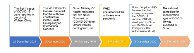
A COVID-19 deterministic compartmental mathematical model with different types of quarantine and isolation is proposed to investigate their role in the disease transmission dynamics. The quarantine compartment is subdivided into short and long quarantine classes, and the isolation compartment is subdivided into tested and non-tested home-isolated individuals and institutionally isolated individuals. The proposed model has been fully analyzed. The analysis includes the positivity and boundedness of solutions, calculation of the control reproduction number and its relation to all transmission routes, existence and stability analysis of disease-free and endemic equilibrium points and bifurcation analysis. The model parameters have been estimated using a dataset for Oman. Using the fitted parameters, the estimated values of the control reproduction number and the contribution of all transmission routes to the reproduction number have been calculated. Sensitivity analysis of the control reproduction number to model parameters has also been performed. Finally, numerical simulations to demonstrate the effect of some model parameters related to the different types of quarantine and isolation on the disease transmission dynamics have been carried out, and the results have been demonstrated graphically.
- COVID-19,
- quarantine,
- isolation,
- reproduction number,
- stability analysis,
- bifurcation analysis,
- sensitivity analysis
Citation: Maryam Al-Yahyai, Fatma Al-Musalhi, Ibrahim Elmojtaba, Nasser Al-Salti. Mathematical analysis of a COVID-19 model with different types of quarantine and isolation[J]. Mathematical Biosciences and Engineering, 2023, 20(1): 1344-1375. doi: 10.3934/mbe.2023061

Related Papers:

Abstract

A COVID-19 deterministic compartmental mathematical model with different types of quarantine and isolation is proposed to investigate their role in the disease transmission dynamics. The quarantine compartment is subdivided into short and long quarantine classes, and the isolation compartment is subdivided into tested and non-tested home-isolated individuals and institutionally isolated individuals. The proposed model has been fully analyzed. The analysis includes the positivity and boundedness of solutions, calculation of the control reproduction number and its relation to all transmission routes, existence and stability analysis of disease-free and endemic equilibrium points and bifurcation analysis. The model parameters have been estimated using a dataset for Oman. Using the fitted parameters, the estimated values of the control reproduction number and the contribution of all transmission routes to the reproduction number have been calculated. Sensitivity analysis of the control reproduction number to model parameters has also been performed. Finally, numerical simulations to demonstrate the effect of some model parameters related to the different types of quarantine and isolation on the disease transmission dynamics have been carried out, and the results have been demonstrated graphically.

References

[1]	Q. Li, X. Guan, P. Wu, X. Wang, L. Zhou, Y. Tong, et al., Early transmission dynamics in Wuhan, China, of novel coronavirus–infected pneumonia, N. Engl. J. Med., 382 (2020), 1199–1207. https://doi.org/10.1056/NEJMoa2001316 doi: 10.1056/NEJMoa2001316
[2]	R. Dutta, L. Buragohain, P. Borah, Analysis of codon usage of severe acute respiratory syndrome corona virus 2 (SARS-CoV-2) and its adaptability in dog, Virus Res., 288 (2020), 1–9. https://doi.org/10.1016/j.virusres.2020.198113 doi: 10.1016/j.virusres.2020.198113
[3]	Y. C. Cao, Q. X. Deng, S. X. Dai, Remdesivir for severe acute respiratory syndrome coronavirus 2 causing COVID-19: An evaluation of the evidence, Travel Med. Infect. Dis., 35 (2020), 1–6. https://doi.org/10.1016/j.tmaid.2020.101647 doi: 10.1016/j.tmaid.2020.101647
[4]	World Health Organization, COVID 19 Public Health Emergency of International Concern (PHEIC). Global research and innovation forum: towards a research roadmap, 2020.
[5]	World Health Organization, Coronavirus Disease (COVID-19), 2021. Available from: https://www.who.int/emergencies/diseases/novel-coronavirus-2019/situation-reports.
[6]	Oman Observer, Coronavirus, 2021. Available from: https://www.omanobserver.om/article/15089/CORONAVIRUS/hm-issues-orders-to-set-up-committee-on-COVID-19.
[7]	S. Kashte, A. Gulbake, S. F. El-Amin III, A. Gupta, COVID-19 vaccines: rapid development, implications, challenges and future prospects, Human cell, 34 (2021), 711–733. https://doi.org/10.1007/s13577-021-00512-4 doi: 10.1007/s13577-021-00512-4
[8]	M. S. Aronna, R. Guglielmi, L. M. Moschen, A model for COVID-19 with isolation, quarantine and testing as control measures, Epidemics, 34 (2021), 100437. https://doi.org/10.1016/j.epidem.2021.100437 doi: 10.1016/j.epidem.2021.100437
[9]	A. Džiugys, M. Bieliūnas, G. Skarbalius, E. Misiulis, R. Navakas, Simplified model of COVID-19 epidemic prognosis under quarantine and estimation of quarantine effectiveness, Chaos Solitons Fractals, 140 (2020), 1–11. https://doi.org/10.1016/j.chaos.2020.110162 doi: 10.1016/j.chaos.2020.110162
[10]	A. Varghese, S. Kolamban, V. Sherimon, E. M. Lacap, S. S. Ahmed, J. P. Sreedhar, et al., SEAMHCRD deterministic compartmental model based on clinical stages of infection for COVID-19 pandemic in Sultanate of Oman, Sci. Rep., 11 (2021), 1–19. https://doi.org/10.1038/s41598-021-91114-5 doi: 10.1038/s41598-021-91114-5
[11]	N. Al-Salti, I. M. Elmojtaba, J. Mesquita, D. Pastore, M. Al-Yahyai Maryam. Analysis of infectious disease problems (COVID-19) and their global impact, Springer Nature, (2021), 219–244.
[12]	Z. Memon, S. Qureshi, B. R. Memon, Assessing the role of quarantine and isolation as control strategies for COVID-19 outbreak: a case study, Chaos Solitons Fractals, 144 (2021), 1–9. https://doi.org/10.1016/j.chaos.2021.110655 doi: 10.1016/j.chaos.2021.110655
[13]	M. A. Khan, A. Atangana, E. Alzahrani, Fatmawati, The dynamics of COVID-19 with quarantined and isolation, Adv. Differ. Equations, 1 (2020), 1–22. https://doi.org/10.1186/s13662-020-02882-9 doi: 10.1186/s13662-020-02882-9
[14]	B. Tang, F. Xia, S. Tang, N. L. Bragazzi, Q. Li, X. Sun, et al., The effectiveness of quarantine and isolation determine the trend of the COVID-19 epidemics in the final phase of the current outbreak in China, Int. J. Infect. Dis., 95 (2020), 288–293. https://doi.org/10.1016/j.ijid.2020.03.018 doi: 10.1016/j.ijid.2020.03.018
[15]	M. Ali, S. T. H. Shah, M. Imran, A. Khan, The role of asymptomatic class, quarantine and isolation in the transmission of COVID-19, J. Biol. Dyn., 149 (2020), 389–408. https://doi.org/10.1080/17513758.2020.1773000 doi: 10.1080/17513758.2020.1773000
[16]	Y. Gu, S. Ullah, M. A. Khan, M. Y. Alshahrani, M. Abohassan, M. B. Riaz, Mathematical modeling and stability analysis of the COVID-19 with quarantine and isolation, Results Phys., 34 (2022), 105284. https://doi.org/10.1016/j.rinp.2022.105284 doi: 10.1016/j.rinp.2022.105284
[17]	S. S. Nadim, I. Ghosh, J. Chattopadhyay, Short-term predictions and prevention strategies for COVID-19: a model-based study, Appl. Math. Comput., 404 (2021), 1–19. https://doi.org/10.1016/j.amc.2021.126251 doi: 10.1016/j.amc.2021.126251
[18]	C. N. Ngonghala, E. Iboi, S. Eikenberry, M. Scotch, C. R. MacIntyre, M. H. Bonds, et al., Mathematical assessment of the impact of non-pharmaceutical interventions on curtailing the 2019 novel Coronavirus, Math. Biosci., 325 (2020), 108364. https://doi.org/10.1016/j.mbs.2020.108364 doi: 10.1016/j.mbs.2020.108364
[19]	M. A. Oud, A. Ali, H. Alrabaiah, S. Ullah, M. A. Khan, S. Islam, A fractional order mathematical model for COVID-19 dynamics with quarantine, isolation, and environmental viral load, Adv. Differ. Equations, 2021 (2021), 1–19. https://doi.org/10.1186/s13662-021-03265-4 doi: 10.1186/s13662-021-03265-4
[20]	W. Ma, Y. Zhao, L. Guo, Y. Chen, Qualitative and quantitative analysis of the COVID-19 pandemic by a two-side fractional-order compartmental model, ISA Trans., 124 (2022), 144–156. https://doi.org/10.1016/j.isatra.2022.01.008 doi: 10.1016/j.isatra.2022.01.008
[21]	N. Ma, W. Ma, Z. Li, Multi-Model selection and analysis for COVID-19, Fractal Fractional, 5 (2021), 1–12. https://doi.org/10.3390/fractalfract5030120 doi: 10.3390/fractalfract5030120
[22]	H. Mohammadi, S. Rezapour, A. Jajarmi, On the fractional SIRD mathematical model and control for the transmission of COVID-19: the first and the second waves of the disease in Iran and Japan, ISA Trans., 124 (2022), 103–114. https://doi.org/10.1016/j.isatra.2021.04.012 doi: 10.1016/j.isatra.2021.04.012
[23]	D. Baleanu, M. H. Abadi, A. Jajarmi, K. Z. Vahid, J. J. Nieto, A new comparative study on the general fractional model of COVID-19 with isolation and quarantine effects, Alexandria Eng. J., 61(6) (2022), 4779–4791. https://doi.org/10.1016/j.aej.2021.10.030 doi: 10.1016/j.aej.2021.10.030
[24]	M. R. Islam, A. Peace, D. Medina, T. Oraby, Integer versus fractional order SEIR deterministic and stochastic models of measles, Int. J. Environ. Res. Public Health, 17 (2020), 1–19. https://doi.org/10.3390/ijerph17062014 doi: 10.3390/ijerph17062014
[25]	P. van den Driessche, J. Watmough, Reproduction numbers and sub-threshold endemic equilibria for compartmental models of disease transmission, Mathematical biosciences, 180(1-2) (2002), 29–48. https://doi.org/10.1016/S0025-5564(02)00108-6 doi: 10.1016/S0025-5564(02)00108-6
[26]	Z. Shuai, P. van den Driessche, Global stability of infectious disease models using Lyapunov functions, SIAM J. Appl. Math., 73 (2013), 1513–1532. https://doi.org/10.1016/10.1137/120876642 doi: 10.1016/10.1137/120876642
[27]	J. P. LaSalle, The Stability of Dynamical Systems, Society for Industrial and Applied Mathematics, 1976.
[28]	C. Castillo-Chavez, B. Song, Dynamical models of tuberculosis and their applications, Math. Biosci. Eng., 1 (2004), 361–404. https://doi.org/10.3934/mbe.2004.1.361 doi: 10.3934/mbe.2004.1.361
[29]	A. Dhooge, W. Govaerts, Y. A. Kuznetsov, H. G. E. Meijer, B. Sautois, New features of the software MatCont for bifurcation analysis of dynamical systems, Math. Comput. Model. Dyn. Syst., 14 (2008), 147–175. https://doi.org/10.1080/13873950701742754 doi: 10.1080/13873950701742754
[30]	Oman VS Covid, The government official account for the efforts of countering COVID-19, 2021. Available from: https://twitter.com/OmanVSCovid19.
[31]	H. P. Gavin, The Levenberg-Marquardt algorithm for nonlinear least squares curve-fitting problems, Mathematics, 19 (2019), 1–19.
[32]	S. A. Lauer, Y. T. Grantz, Q. Bi, F. K. Jones, Q. Zheng, H. R. Meredith, et al., The incubation period of coronavirus disease 2019 (COVID-19) from publicly reported confirmed cases: estimation and application, Ann. Intern. Med., 172 (2020), 577-582. https://doi.org/10.7326/M20-0504 doi: 10.7326/M20-0504
[33]	J. Zhang, M. Litvinova, W. Wang, Y. Wang, X. Deng, X. Chen, et al., Evolving epidemiology and transmission dynamics of coronavirus disease 2019 outside Hubei province, China: A descriptive and modelling study, Lancet Infect. Dis., 20 (2020), 793–802. https://doi.org/10.1016/S1473-3099(20)30230-9 doi: 10.1016/S1473-3099(20)30230-9
[34]	S. Sanche, Y. T. Lin, C. Xu, E. Romero-Severson, N. Hengartner, R. Ke, High contagiousness and rapid spread of severe acute respiratory syndrome coronavirus 2, Emerging Infect. Dis., 26 (2020), 1470–1477. https://doi.org/10.3201/eid2607.200282 doi: 10.3201/eid2607.200282
[35]	M. Casey-Bryars, J. Griffin, C. McAloon, A. Byrne, J. Madden, D. Mc Evoy, et al., Presymptomatic transmission of SARS-CoV-2 infection: a secondary analysis using published data, BMJ Open, 11 (2021), e041240. http://dx.doi.org/10.1136/bmjopen-2020-041240 doi: 10.1136/bmjopen-2020-041240
[36]	D. Buitrago-Garcia, D. Egli-Gany, M. J. Counotte, S. Hossmann, H. Imeri, A. M. Ipekci, et al., Occurrence and transmission potential of asymptomatic and presymptomatic SARS-CoV-2 infections: A living systematic review and meta-analysis, PLoS Med., 17 (2020), e1003346. https://doi.org/10.1371/journal.pmed.1003346 doi: 10.1371/journal.pmed.1003346

Reader Comments

Your name:*

Email:*
© 2023 the Author(s), licensee AIMS Press. This is an open access article distributed under the terms of the Creative Commons Attribution License (http://creativecommons.org/licenses/by/4.0)