Analysis of the COVID-19 model with self-protection and isolation measures affected by the environment

Jiangbo Hao; Lirong Huang; Maoxing Liu; Yangjun Ma; Jiangbo Hao; Lirong Huang; Maoxing Liu; Yangjun Ma

doi:10.3934/mbe.2024213

Mathematical Biosciences and Engineering

2024, Volume 21, Issue 4: 4835-4852. doi: 10.3934/mbe.2024213

Previous Article Next Article

Research article

Analysis of the COVID-19 model with self-protection and isolation measures affected by the environment

1.
School of Mathematics and Statistics, Chongqing Jiaotong University, Chongqing 400074, China
2.
School of Biological Engineering, Guangdong Medical University, Dongguan 523109, China
3.
College of Science, Beijing University of Civil Engineering and Architecture, Beijing 102616, China

Academic Editor: Libin Rong

Received: 03 December 2023 Revised: 21 February 2024 Accepted: 22 February 2024 Published: 29 February 2024

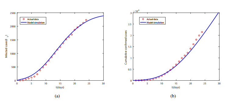
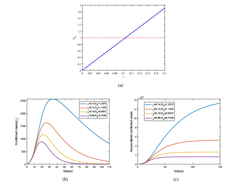
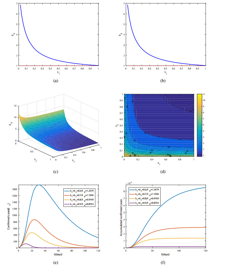
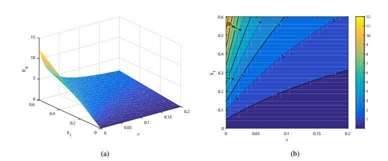
Since the global outbreak of COVID-19, the virus has continuously mutated and can survive in the air for long periods of time. This paper establishes and analyzes a model of COVID-19 with self-protection and quarantine measures affected by viruses in the environment to investigate the influence of viruses in the environment on the spread of the outbreak, as well as to develop a rational prevention and control measure to control the spread of the outbreak. The basic reproduction number was calculated and Lyapunov functions were constructed to discuss the stability of the model equilibrium points. The disease-free equilibrium point was proven to be globally asymptotically stable when $ R_0 < 1 $, and the endemic equilibrium point was globally asymptotically stable when $ R_0 > 1 $. The model was fitted using data from COVID-19 cases in Chongqing between November 1 to November 25, 2022. Based on the numerical analysis, the following conclusion was obtained: clearing the virus in the environment and strengthening the isolation measures for infected people can control the epidemic to a certain extent, but enhancing the self-protection of individuals can be more effective in reducing the risk of being infected and controlling the transmission of the epidemic, which is more conducive to the practical application.
- COVID-19,
- stability analysis,
- isolation measures,
- self-protection
Citation: Jiangbo Hao, Lirong Huang, Maoxing Liu, Yangjun Ma. Analysis of the COVID-19 model with self-protection and isolation measures affected by the environment[J]. Mathematical Biosciences and Engineering, 2024, 21(4): 4835-4852. doi: 10.3934/mbe.2024213

Related Papers:

Abstract

Since the global outbreak of COVID-19, the virus has continuously mutated and can survive in the air for long periods of time. This paper establishes and analyzes a model of COVID-19 with self-protection and quarantine measures affected by viruses in the environment to investigate the influence of viruses in the environment on the spread of the outbreak, as well as to develop a rational prevention and control measure to control the spread of the outbreak. The basic reproduction number was calculated and Lyapunov functions were constructed to discuss the stability of the model equilibrium points. The disease-free equilibrium point was proven to be globally asymptotically stable when $ R_0 < 1 $, and the endemic equilibrium point was globally asymptotically stable when $ R_0 > 1 $. The model was fitted using data from COVID-19 cases in Chongqing between November 1 to November 25, 2022. Based on the numerical analysis, the following conclusion was obtained: clearing the virus in the environment and strengthening the isolation measures for infected people can control the epidemic to a certain extent, but enhancing the self-protection of individuals can be more effective in reducing the risk of being infected and controlling the transmission of the epidemic, which is more conducive to the practical application.

References

[1]	J. Cohen, D. Normile, New SARS-like virus in China triggers alarm, Science, 367 (2020), 234–235. https://doi.org/10.1126/science.367.6475.234 doi: 10.1126/science.367.6475.234
[2]	C. Eastin, T. Eastin, Risk factors as sociated with acute respiratory distress syndrome and death in patients with coronavirus disease 2019 pneumonia in Wuhan, China, J. Emerg. Med., 367 (2020), 234–235. https://doi.org/10.1016/j.jemermed.2020.04.007 doi: 10.1016/j.jemermed.2020.04.007
[3]	C. Eastin, T. Eastin, Clinical characteristics of coronavirus disease 2019 in China, J. Emerg. Med., 58 (2020), 711–712. https://doi.org/10.1016/j.jemermed.2020.04.004 doi: 10.1016/j.jemermed.2020.04.004
[4]	S. Richardson, J. S. Hirsch, M. Narasimhan, Presenting characteristics, comorbidities, and outcomes among 5700 patients hospitalized with COVID-19 in the New York City area, Jama, 323 (2020), 2052–2059. https://doi.org/10.1001/jama.2020.6775 doi: 10.1001/jama.2020.6775
[5]	Z. Kolahchi, M. Domenico, L. Uddin, V. Cauda, N. Rezaei, COVID-19 and its global economic impact, in Coronavirus Disease-COVID-19, 1318 (2021), 825–837. https://doi.org/10.1007/978-3-030-63761-3_46
[6]	S. J. Thomas, E. D. Moreira, N. Kitchin, J. Absalon, A. Gurtman, S. Lockhart, et al., Safety and efficacy of the BNT162b2 mRNA Covid-19 vaccine through 6 months, New. Engl. J. Med., 385 (2021), 1761–1773. https://doi.org/10.1056/NEJMOA2110345 doi: 10.1056/NEJMOA2110345
[7]	W. Xu, H. Shu, L. Wang, X. Wang, J. Watmough, The importance of quarantine: modelling the COVID-19 testing process, J. Math. Biol., 86 (2023), 81. https://doi.org/10.1007/s00285-023-01916-6 doi: 10.1007/s00285-023-01916-6
[8]	M. Ali, S. T. H. Shah, M. Imran, A. Khan, The role of asymptomatic class, quarantine and isolation in the transmission of COVID-19, J. Biol. Dyn., 14 (2020), 389–408. https://doi.org/10.1080/17513758.2020.1773000 doi: 10.1080/17513758.2020.1773000
[9]	M. A. A. Oud, A. Ali, H. Alrabaiah, S. Ullah, A fractional order mathematical model for COVID-19 dynamics with quarantine, isolation, and environmental viral load, Adv. Differ. Equations, 2021 (2021), 1–19. https://doi.org/10.1186/s13662-021-03265-4 doi: 10.1186/s13662-021-03265-4
[10]	M. A. Khan, A. Atangana, E. Alzahrani, The dynamics of COVID-19 with quarantined and isolation, Adv. Differ. Equations, 2020 (2020), 425. https://doi.org/10.1186/s13662-020-02882-9 doi: 10.1186/s13662-020-02882-9
[11]	Q. Pan, T. Gao, M. He, Influence of isolation measures for patients with mild symptoms on the spread of COVID-19, Chaos, Solitons Fractals, 139 (2020), 110022. https://doi.org/10.1016/j.chaos.2020.110022 doi: 10.1016/j.chaos.2020.110022
[12]	Y. Guo, T. Li, Modeling the competitive transmission of the Omicron strain and Delta strain of COVID-19, J. Math. Anal. Appl., 526 (2023), 127283–127283. https://doi.org/10.1016/j.jmaa.2023.127283 doi: 10.1016/j.jmaa.2023.127283
[13]	J. Zhang, Y. Li, M. Yao, J. Zhang, H. Zhu, Z. Jin, Analysis of the relationship between transmission of COVID-19 in Wuhan and soft quarantine intensity in susceptible population, Acta. Math. Appl. Sin., 43 (2020), 162–173.
[14]	B. Tang, X. Wang, Q. Li, Estimation of the transmission risk of the 2019-nCoV and its implication for public health interventions, J. Clin. Med. Res., 9 (2020), 462. https://doi.org/10.3390/jcm9020462 doi: 10.3390/jcm9020462
[15]	R. Yuan, Y. Ma, C. Shen, Global dynamics of COVID-19 epidemic model with recessive infection and isolation, Math. Biosci. Eng., 18 (2021), 1833–1844. https://doi.org/10.3934/mbe.2021095 doi: 10.3934/mbe.2021095
[16]	M. Al-Yahyai, F. Al-Musalhi, I. Elmojtaba, N. Al-Salti, Mathematical analysis of a COVID-19 model with different types of quarantine and isolation, Math. Biosci. Eng., 20 (2023), 1344–1375 https://doi.org/10.3934/mbe.2023061 doi: 10.3934/mbe.2023061
[17]	T. Li, Y. Guo, Modeling and optimal control of mutated COVID-19 (Delta strain) with imperfect vaccination, Chaos, Solitons Fractals, 156 (2022), 111825. https://doi.org/10.1016/j.chaos.2022.111825 doi: 10.1016/j.chaos.2022.111825
[18]	X. Chen, R. Wang, D. Yang, J. Xian, Q. Li, Effects of the Awareness-Driven Individual Resource Allocation on the Epidemic Dynamics, Complexity, 2020 (2020), 1–12. https://doi.org/10.1155/2020/8861493 doi: 10.1155/2020/8861493
[19]	Y. Guo, T. Li, Modeling the transmission of second-wave COVID-19 caused by imported cases: A case study, Math. Methods Appl. Sci., 45 (2022), 8096–8114. https://doi.org/10.1002/mma.8041 doi: 10.1002/mma.8041
[20]	M. S. Ullah, M. Higazy, K. M. A. Kabir, Modeling the epidemic control measures in overcoming COVID-19 outbreaks: A fractional-order derivative approach, Chaos, Solitons Fractals, 155 (2022), 111636. https://doi.org/10.1016/j.chaos.2021.111636 doi: 10.1016/j.chaos.2021.111636
[21]	H. Huo, S. Hu, H. Xiang, Traveling wave solution for a diffusion SEIR epidemic model with self-protection and treatment, Electron. Res. Arch., 29 (2021), 2325–2358. https://doi.org/10.3934/era.2020118 doi: 10.3934/era.2020118
[22]	S. Lai, N. W. Ruktanonchai, L. Zhou, O. Prosper, W. Luo, J. R. Floyd, et al., Effect of non-pharmaceutical interventions to contain COVID-19 in China, Nature, 585 (2020), 410–413. https://doi.org/10.1038/s41586-020-2293-x doi: 10.1038/s41586-020-2293-x
[23]	L. Hu, L. Nie, Dynamic modeling and analysis of COVID‐19 in different transmission process and control strategies, Math. Methods Appl. Sci., 44 (2021), 409–1422. https://doi.org/10.1002/mma.6839 doi: 10.1002/mma.6839
[24]	World Health Organization, Listings of WHO's response to COVID-19, 2020. Available from: https://www.who.int/news/item/29-06-2020-covidtimeline
[25]	A. Wang, X. Zhang, R. Yan, D. Bai, J. He, Evaluating the impact of multiple factors on the control of COVID-19 epidemic: A modelling analysis using India as a case study, Math. Biosci. Eng., 20 (2023), 6237–6272. https://doi.org/10.3934/mbe.2023269 doi: 10.3934/mbe.2023269
[26]	S. Musa, A. Yusuf, S. Zhao, Z. Abdullahi, H. Abu-Odah, F. T. Saad, et al., Transmission dynamics of COVID-19 pandemic with combined effects of relapse, reinfection and environmental contribution: A modeling analysis, Results Phys., 38 (2022), 105653. https://doi.org/10.1016/j.rinp.2022.105653 doi: 10.1016/j.rinp.2022.105653
[27]	Y. Bai, L. Yao, T. Wei, Presumed asymptomatic carrier transmission of COVID-19, Jama, 323 (2020), 1406–1407. https://doi.org/10.1001/jama.2020.2565 doi: 10.1001/jama.2020.2565
[28]	O. Diekmann, J. A. P. Heesterbeek, J. A. J. Metz, On the definition and the computation of the basic reproduction ratio $R_0$ in models for infectious diseases in heterogeneous populations, J. Math. Biol., 28 (1990), 365–382. https://doi.org/10.1007/BF00178324 doi: 10.1007/BF00178324
[29]	P. van den Driessche., J. Watmough, Reproduction numbers and sub-threshold endemic equilibria for compartmental models of disease transmission, Math. Biosci., 180 (2002), 29–48. https://doi.org/10.1016/S0025-5564(02)00108-6 doi: 10.1016/S0025-5564(02)00108-6
[30]	J. P. LaSalle, The Stability of Dynamical Systems, Society for industrial and applied mathematics, USA, 1976. http://dx.doi.org/10.1137/1.9781611970432
[31]	Chongqing Municipal Health Commission. Available from: https://wsjkw.cq.gov.cn/.
[32]	Chongqing Center for Disease Control and Prevention. Available from: https://www.cqcdc.org/.
[33]	Chongqing Municipal People's Government. Available from: http://www.cq.gov.cn/.
[34]	B. Li, A. Deng, K. Li, Y. Hu, Z. Li, Y. Shi, et al., Viral infection and transmission in a large, well-traced outbreak caused by the SARS-CoV-2 Delta variant, Nat. Commun., 13 (2020), 460. https://doi.org/10.1038/s41467-022-28089-y doi: 10.1038/s41467-022-28089-y

Reader Comments

Your name:*

Email:*
© 2024 the Author(s), licensee AIMS Press. This is an open access article distributed under the terms of the Creative Commons Attribution License (http://creativecommons.org/licenses/by/4.0)