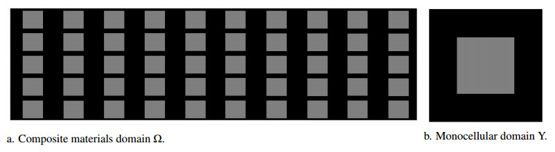
In this paper, a topology optimization algorithm for the mechanical-electrical coupling problem of periodic composite materials is studied. Firstly, the homogenization problem of the mechanical-electrical coupling topology optimization problem of periodic composite materials is established by the multi-scale asymptotic expansion method. Secondly, the topology optimization algorithm for the mechanical-electrical coupling problem of periodic composite materials is constructed by finite element method, solid isotropic material with penalisation method and homogenization method. Finally, numerical results show that the proposed algorithm is effective to calculate the optimal structure of the periodic composite cantilever beam under the influence of the mechanical-electrical coupling.
Citation: Ziqiang Wang, Chunyu Cen, Junying Cao. Topological optimization algorithm for mechanical-electrical coupling of periodic composite materials[J]. Electronic Research Archive, 2023, 31(5): 2689-2707. doi: 10.3934/era.2023136
In this paper, a topology optimization algorithm for the mechanical-electrical coupling problem of periodic composite materials is studied. Firstly, the homogenization problem of the mechanical-electrical coupling topology optimization problem of periodic composite materials is established by the multi-scale asymptotic expansion method. Secondly, the topology optimization algorithm for the mechanical-electrical coupling problem of periodic composite materials is constructed by finite element method, solid isotropic material with penalisation method and homogenization method. Finally, numerical results show that the proposed algorithm is effective to calculate the optimal structure of the periodic composite cantilever beam under the influence of the mechanical-electrical coupling.

| [1] |
A. C. Eringen, Theory of nonlocal piezoelectricity, J. Math. Phys., 25 (1984), 717–727. https://doi.org/10.1063/1.526180 doi: 10.1063/1.526180

|
| [2] |
J. S. Yang, R. C. Batra, Conservation laws in linear piezoelectricity, Eng. Fract. Mech., 51 (1995), 1041–1047. https://doi.org/10.1016/0013-7944(94)00271-I doi: 10.1016/0013-7944(94)00271-I
|
| [3] |
M. Deng, Y. Feng, Two-scale finite element for piezoelectric problem in periodic structure, Appl. Math. Mech., 32 (2011), 1525–1540. https://doi.org/10.1007/s10483-011-1521-7 doi: 10.1007/s10483-011-1521-7
|
| [4] |
J. Telega, S. Bytner, Piezoelectricity with polarization gradient: homogenization, Mech. Res. Commun., 29 (2002), 53–59. https://doi.org/10.1016/S0093-6413(02)00228-8 doi: 10.1016/S0093-6413(02)00228-8
|
| [5] |
G. Allaire, E. Bonnetier, G. Francfort, F. Jouve, Shape optimization by the homogenization method, Numer. Math., 76 (1997), 27–68. https://doi.org/10.1007/s002110050253 doi: 10.1007/s002110050253
|
| [6] |
M. Zhou, D. Geng, Multi-scale and multi-material topology optimization of channel-cooling cellular structures for thermomechanical behaviors, Comput. Methods Appl. Mech. Eng., 383 (2021), 113896. https://doi.org/10.1016/j.cma.2021.113896 doi: 10.1016/j.cma.2021.113896
|
| [7] |
X. Zhao, M. Zhou, Y. Liu, M. Ding, P. Hu, P. Zhu, Topology optimization of channel cooling structures considering thermomechanical behavior, Struct. Multidiscip. Optim., 59 (2019), 613–632. https://doi.org/10.1007/s00158-018-2087-z doi: 10.1007/s00158-018-2087-z
|
| [8] |
L. Ling, J. Yan, G. Cheng, Optimum structure with homogeneous optimum truss-like material, Comput. Struct., 86 (2008), 1417–1425. https://doi.org/10.1016/j.compstruc.2007.04.030 doi: 10.1016/j.compstruc.2007.04.030
|
| [9] |
A. Homayouni-Amlashi, A. Mohand-Ousaid, M. Rakotondrabe, Topology optimization of 2DOF piezoelectric plate energy harvester under external in-plane force, J. Micro-Bio Rob., 16 (2020), 65–77. https://doi.org/10.1007/s12213-020-00129-0 doi: 10.1007/s12213-020-00129-0
|
| [10] |
B. Yang, C. Cheng, X. Wang, Z. Meng, A. Homayouni-Amlashi, Reliability-based topology optimization of piezoelectric smart structures with voltage uncertainty, J. Intell. Mater. Syst. Struct., 33 (2022), 1975–1989. https://doi.org/10.1177/1045389X211072197 doi: 10.1177/1045389X211072197
|
| [11] |
L. Xu, G. Cheng, Two-scale concurrent topology optimization with multiple micro materials based on principal stress orientation, Struct. Multidiscip. Optim., 57 (2018), 2093–2107. https://doi.org/10.1007/s00158-018-1916-4 doi: 10.1007/s00158-018-1916-4
|
| [12] |
S. Xu, G. Cheng, Optimum material design of minimum structural compliance under seepage constraint, Struct. Multidiscip. Optim., 41 (2010), 575–587. https://doi.org/10.1007/s00158-009-0438-5 doi: 10.1007/s00158-009-0438-5
|
| [13] |
H. Rodrigues, J. Guedes, M. Bendsoe, Hierarchical optimization of material and structure, Struct. Multidiscip. Optim., 24 (2002), 1–10. https://doi.org/10.1007/s00158-002-0209-z doi: 10.1007/s00158-002-0209-z
|
| [14] |
J. Guedes, N. Kikuchi, Preprocessing and postprocessing for materials based on the homogenization method with adaptive finite element methods, Comput. Methods Appl. Mech. Eng., 83 (1990), 143–198. https://doi.org/10.1016/0045-7825(90)90148-F doi: 10.1016/0045-7825(90)90148-F
|
| [15] |
E. Andreassen, C. Andreasen, How to determine composite material properties using numerical homogenization, Comput. Mater. Sci., 83 (2014), 488–495. https://doi.org/10.1016/j.commatsci.2013.09.006 doi: 10.1016/j.commatsci.2013.09.006
|
| [16] |
G. Cheng, Y. Cai, L. Xu, Novel implementation of homogenization method to predict effective properties of periodic materials, Acta Mech. Sin., 29 (2013), 550–556. https://doi.org/10.1007/s10409-013-0043-0 doi: 10.1007/s10409-013-0043-0
|
| [17] |
Y. Wang, M. Wang, F. Chen, Structure-material integrated design by level sets, Struct. Multidiscip. Optim., 54 (2016), 1145–1156. https://doi.org/10.1007/s00158-016-1430-5 doi: 10.1007/s00158-016-1430-5
|
| [18] |
J. Guest, J. Prvost, Optimizing multifunctional materials: design of microstructures for maximized stiffness and fluid permeability, Int. J. Solids Struct., 43 (2006), 7028–7047. https://doi.org/10.1016/j.ijsolstr.2006.03.001 doi: 10.1016/j.ijsolstr.2006.03.001
|
| [19] |
J. Guest, J. Prvost, Design of maximum permeability material structures, Comput. Methods Appl. Mech. Eng., 196 (2007), 1006–1017. https://doi.org/10.1016/j.cma.2006.08.006 doi: 10.1016/j.cma.2006.08.006
|
| [20] |
Z. Han, Z. Wang, K. Wei, Shape morphing structures inspired by multi-material topology optimized bi-functional metamaterials, Compos. Struct., 300 (2022), 116135. https://doi.org/10.1016/j.compstruct.2022.116135 doi: 10.1016/j.compstruct.2022.116135
|
| [21] |
Z. Han, K. Wei, Multi-material topology optimization and additive manufacturing for metamaterials incorporating double negative indexes of Poissons ratio and thermal expansion, Addit. Manuf., 54 (2022), 102742. https://doi.org/10.1016/j.addma.2022.102742 doi: 10.1016/j.addma.2022.102742
|
| [22] |
M. Costa, A. Sohouli, A. Suleman, Multi-scale and multi-material topology optimization of gradient lattice structures using surrogate models, Compos. Struct., 289 (2022), 115402. https://doi.org/10.1016/j.compstruct.2022.115402 doi: 10.1016/j.compstruct.2022.115402
|
| [23] |
X. Huangy, W. Li, A new multi-material topology optimization algorithm and selection of candidate materials, Comput. Methods Appl. Mech. Eng., 386 (2021), 114114. https://doi.org/10.1016/J.CMA.2021.114114 doi: 10.1016/J.CMA.2021.114114
|
| [24] |
Z. Wang, J. Cui, Second-order two-scale method for bending behavior analysis of composite plate with 3-D periodic configuration and its approximation, Sci. China Math., 57 (2014), 1713–1732. https://doi.org/10.1007/s11425-014-4831-1 doi: 10.1007/s11425-014-4831-1
|
| [25] |
J. Cao, C. Xu, A high order schema for the numerical solution of the fractional ordinary differential equations, J. Comput. Phys., 238 (2013), 154–168. https://doi.org/10.1016/j.jcp.2012.12.013 doi: 10.1016/j.jcp.2012.12.013
|
| [26] |
L. Tian, Z. Wang, J. Cao, A high-order numerical scheme for right Caputo fractional differential equations with uniform accuracy, Electron. Res. Arch., 30 (2022), 3825–3854. https://doi:10.3934/era.2022195 doi: 10.3934/era.2022195
|
| [27] |
C. Wang, J. Zhu, W. Zhang, S. Li, J. Kong, Concurrent topology optimization design of structures and non-uniform parameterized lattice microstructures, Struct. Multidiscip. Optim., 58 (2018), 35–50. https://doi.org/10.1007/s00158-018-2009-0 doi: 10.1007/s00158-018-2009-0
|
| [28] |
P. Gangl, A multi-material topology optimization algorithm based on the topological derivative, Comput. Methods Appl. Mech. Eng., 366 (2020), 113090. https://doi.org/10.1016/j.cma.2020.113090 doi: 10.1016/j.cma.2020.113090
|
| [29] |
Y. Feng, M. Deng, X. Guan, The twoscale asymptotic error analysis for piezoelectric problems in the quasi-periodic structure, Sci. China Phys., Mech. Astron., 56 (2013), 1844–1853. https://doi.org/10.1007/s11433-013-5304-1 doi: 10.1007/s11433-013-5304-1
|
| [30] |
A. Homayouni-Amlashi, T. Schlinquer, A. Mohand-Ousaid, M. Rakotondrabe, 2D topology optimization MATLAB codes for piezoelectric actuators and energy harvester, Struct. Multidiscip. Optim., 63 (2021), 983–1014. https://doi.org/10.1007/s00158-020-02726-w doi: 10.1007/s00158-020-02726-w
|
| [31] |
M. Wang, S. Feng, A. Incecik, G. Krolczyk, Z. Li, Structural fatigue life prediction considering model uncertainties through a novel digital twin-driven approach, Comput. Methods Appl. Mech. Eng., 391 (2022), 114512. https://doi.org/10.1016/j.cma.2021.114512 doi: 10.1016/j.cma.2021.114512
|
| [32] |
S. Feng, X. Han, Z. Li, A. Incecik, Ensemble learning for remaining fatigue life prediction of structures with stochastic parameters: a data-driven approach, Appl. Math. Modell., 101 (2022), 420–431. https://doi.org/10.1016/j.apm.2021.08.033 doi: 10.1016/j.apm.2021.08.033
|
| [33] |
W. Mason, H. Baerwald, Piezoelectric crystals and their applications to ultrasonics, Phys. Today, 4 (1951), 23–24. https://doi.org/10.1063/1.3067231 doi: 10.1063/1.3067231
|


Figures(3) / Tables(3)
Ziqiang Wang, Chunyu Cen, Junying Cao. Topological optimization algorithm for mechanical-electrical coupling of periodic composite materials[J]. Electronic Research Archive, 2023, 31(5): 2689-2707. doi: 10.3934/era.2023136


 DownLoad: