In response-guided dosing (RGD), the goal is to make optimal dosing decisions based on the stochastic evolution of a patient's disease condition. Typically, RGD is formulated as a finite-horizon problem with decision-making occurring over a predetermined time frame. In this paper we relax the latter assumption to allow for the possibility of ending treatment early. This could occur due to remission of the disease or a finding of futility in treatment of the disease. Our framework is formulated as a stochastic dynamic program (DP) where a stop/do-not-stop decision is made in discrete sessions, and if stopping is not chosen, an optimal dose is determined for that session. Numerical simulations for rheumatoid arthritis are presented, and monotonicity of the stop/do-not-stop threshold with respect to time is proven.
Citation: Jakob Kotas. Optimal stopping for response-guided dosing[J]. Networks and Heterogeneous Media, 2019, 14(1): 43-52. doi: 10.3934/nhm.2019003
In response-guided dosing (RGD), the goal is to make optimal dosing decisions based on the stochastic evolution of a patient's disease condition. Typically, RGD is formulated as a finite-horizon problem with decision-making occurring over a predetermined time frame. In this paper we relax the latter assumption to allow for the possibility of ending treatment early. This could occur due to remission of the disease or a finding of futility in treatment of the disease. Our framework is formulated as a stochastic dynamic program (DP) where a stop/do-not-stop decision is made in discrete sessions, and if stopping is not chosen, an optimal dose is determined for that session. Numerical simulations for rheumatoid arthritis are presented, and monotonicity of the stop/do-not-stop threshold with respect to time is proven.

| [1] |
Adaptive Bayesian designs for dose-ranging drug trials. Case Studies in Bayesian Statistics (2002) 5: 99-181. 
|
| [2] |
D. P. Bertsekas, Dynamic Programming and Optimal Control, 4th edition, Athena Scientific, Cambridge, MA, 2012. |
| [3] |
Early virologic response to treatment with peginterferon alfa-2b plus ribavirin in patients with chronic hepatitis C. Hepatology (2003) 38: 645-652.
|
| [4] |
Titration of infliximab treatment in rheumatoid arthritis patients based on response patterns. Rheumatology (2007) 46: 146-149.
|
| [5] | On Stefan's problem and optimal stopping rules for Markov processes. Theory of Probability and its Applications (1966) 4: 541-558. |
| [6] |
Refinement of stopping rules during treatment of hepatitis C genotype 1 infection with boceprevir and peginterferon/ribavirin. Hepatology (2012) 56: 567-575.
|
| [7] | Response-guided dosing for rheumatoid arthritis. IIE Transactions on Healthcare Systems Engineering (2016) 6: 1-21. |
| [8] |
Bayesian learning of dose-response parameters from a cohort under response-guided dosing. European Journal of Operational Research (2018) 265: 328-343.
|
| [9] |
Flare rate in patients with rheumatoid arthritis in low disease activity or remission when tapering or stopping synthetic or biologic DMARD: a systematic review. Journal of Rheumatology (2015) 42: 2012-2022.
|
| [10] |
Down-titration and discontinuation of infliximab, adalimumab and etanercept in established rheumatoid arthritis. Annals of the Rheumatic Diseases (2013) 72: 237.
|
| [11] |
Infliximab discontinuation in Crohn's disease patients in stable remission on combined therapy with immunosuppressors: a prospective ongoing cohort study. Gastroenterology (2009) 136: A146.
|
| [12] |
Outcome of infliximab discontinuation in IBD patients and therapy rechallenging in relapsers: Single centre preliminary data. Journal of Crohn's and Colitis (2014) 8: S232-S233.
|
| [13] | A Bayesian decision-theoretic dose-finding trial. Decision Analysis (2006) 3: 197-207. |
| [14] | (1994) Markov Decision Processes: Discrete Stochastic Dynamic Programming. New York: John Wiley & Sons, Inc.. |
| [15] |
Response-guided telaprevir combination treatment for hepatitis C virus infection. The New England Journal of Medicine (2011) 365: 1014-1024.
|
| [16] | (2008) Optimal Stopping Rules. Berlin Heidelberg: Springer-Verlag. |
| [17] |
Dose-response modeling of continuous endpoints. Toxicological Sciences (2002) 66: 298-312.
|
| [18] |
Effect of interleukin-6 receptor inhibition with tocilizumab in patients with rheumatoid arthritis (OPTION study): a double-blind, placebo-controlled, randomised trial. The Lancet (2008) 371: 987-997.
|
| [19] |
Meta-analysis- maintenance of remission following discontinuation of infliximab in patients with Crohn's disease. Gastroenterology (2013) 144: S637.
|
| [20] |
Response-guided peginterferon therapy in hepatitis B e antigen-positive chronic hepatitis B using serum hepatitis B surface antigen levels. Hepatology (2013) 58: 872-880.
|
| [21] |
Prediction of sustained response to peginterferon alfa-2b for hepatitis B e antigen-positive chronic hepatitis B using on-treatment hepatitis B surface antigen decline. Hepatology (2012) 52: 1251-1257.
|
| [22] | Randomised placebo-controlled study of stopping second-line drugs in rheumatoid arthritis. The Lancet (1996) 347: 347-352. |
| [23] | Down-titration and discontinuation of infliximab in rheumatoid arthritis patients with stable low disease activity and stable treatment: an observational cohort study. Annals of Rheumatoid Disease (2012) 71: 1849-1854. |
| [24] |
Down-titration and discontinuation strategies of tumor necrosis factor-blocking agents for rheumatoid arthritis patients with low disease activity. Cochrane Database of Systematic Reviews (2013) 9:.
|
Figures(2)
Jakob Kotas. Optimal stopping for response-guided dosing[J]. Networks and Heterogeneous Media, 2019, 14(1): 43-52. doi: 10.3934/nhm.2019003

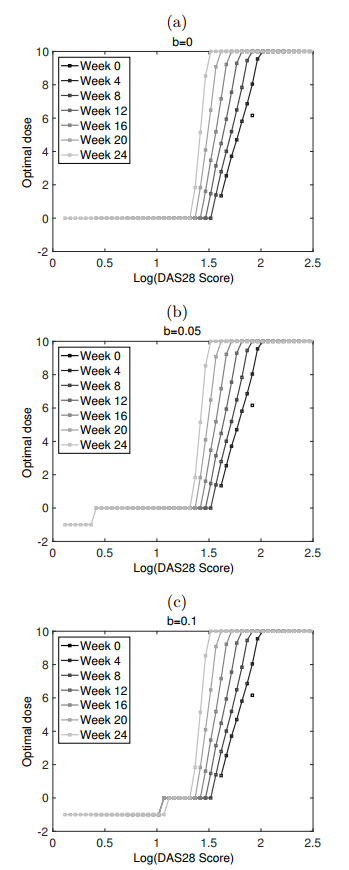
Optimal policy of tocilizumab dosing for rheumatoid arthritis. The cost functions are
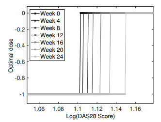
Optimal policy with the cost function


 DownLoad: