The parabolic-elliptic Keller-Segel equation with sensitivity saturation, because of its pattern formation ability, is a challenge for numerical simulations. We provide two finite-volume schemes that are shown to preserve, at the discrete level, the fundamental properties of the solutions, namely energy dissipation, steady states, positivity and conservation of total mass. These requirements happen to be critical when it comes to distinguishing between discrete steady states, Turing unstable transient states, numerical artifacts or approximate steady states as obtained by a simple upwind approach.
These schemes are obtained either by following closely the gradient flow structure or by a proper exponential rewriting inspired by the Scharfetter-Gummel discretization. An interesting fact is that upwind is also necessary for all the expected properties to be preserved at the semi-discrete level. These schemes are extended to the fully discrete level and this leads us to tune precisely the terms according to explicit or implicit discretizations. Using some appropriate monotonicity properties (reminiscent of the maximum principle), we prove well-posedness for the scheme as well as all the other requirements. Numerical implementations and simulations illustrate the respective advantages of the three methods we compare.
Citation: Luis Almeida, Federica Bubba, Benoît Perthame, Camille Pouchol. Energy and implicit discretization of the Fokker-Planck and Keller-Segel type equations[J]. Networks and Heterogeneous Media, 2019, 14(1): 23-41. doi: 10.3934/nhm.2019002
The parabolic-elliptic Keller-Segel equation with sensitivity saturation, because of its pattern formation ability, is a challenge for numerical simulations. We provide two finite-volume schemes that are shown to preserve, at the discrete level, the fundamental properties of the solutions, namely energy dissipation, steady states, positivity and conservation of total mass. These requirements happen to be critical when it comes to distinguishing between discrete steady states, Turing unstable transient states, numerical artifacts or approximate steady states as obtained by a simple upwind approach.
These schemes are obtained either by following closely the gradient flow structure or by a proper exponential rewriting inspired by the Scharfetter-Gummel discretization. An interesting fact is that upwind is also necessary for all the expected properties to be preserved at the semi-discrete level. These schemes are extended to the fully discrete level and this leads us to tune precisely the terms according to explicit or implicit discretizations. Using some appropriate monotonicity properties (reminiscent of the maximum principle), we prove well-posedness for the scheme as well as all the other requirements. Numerical implementations and simulations illustrate the respective advantages of the three methods we compare.

| [1] |
A continuum approach to modelling cell-cell adhesion. Journal of Theoretical Biology (2006) 243: 98-113. 
|
| [2] |
Particle interactions mediated by dynamical networks: Assessment of macroscopic descriptions. Journal of Nonlinear Science (2018) 28: 235-268.
|
| [3] |
Blow-up in multidimensional aggregation equations with mildly singular interaction kernels. Nonlinearity (2009) 22: 683-710.
|
| [4] |
A finite volume scheme for nonlinear degenerate parabolic equations. SIAM Journal on Scientific Computing (2012) 34: 559-583.
|
| [5] |
Convergence of the mass-transport steepest descent scheme for the subcritical Patlak-Keller-Segel model. SIAM Journal on Numerical Analysis (2008) 46: 691-721.
|
| [6] | Two-dimensional Keller-Segel model: Optimal critical mass and qualitative properties of the solutions. Electronic Journal of Differential Equations (2006) 2006: 1-32. |
| [7] |
F. Bouchut, Nonlinear Stability of Finite Volume Methods for Hyperbolic Conservation Laws and Well-balanced Schemes for Sources, Birkhäuser, 2004. |
| [8] |
A finite-volume method for nonlinear nonlocal equations with a gradient flow structure. Communications in Computational Physics (2015) 17: 233-258.
|
| [9] |
J. A. Carrillo, N. Kolbe and M. Lukacova-Medvidova, A hybrid mass-transport finite element method for Keller-Segel type systems, preprint, arXiv: 1709.07394, (2017). |
| [10] |
Zoology of a non-local cross-diffusion model for two species. SIAM Journal on Applied Mathematics (2018) 78: 1078-1104.
|
| [11] | Quasilinear non-uniformly parabolic-elliptic system modelling chemotaxis with volume filling effect. Existence and uniqueness of global-in-time solutions. Topological Methods in Nonlinear Analysis (2007) 29: 361-381. |
| [12] |
Stationary solutions of Keller-Segel type crowd motion and herding models: Multiplicity and dynamical stability. Mathematics and Mechanics of Complex Systems (2015) 3: 211-242.
|
| [13] | Finite volume methods. Handbook of Numerical Analysis (2000) 7: 713-1020. |
| [14] | Volume-filling and quorum-sensing in models for chemosensitive movement. Canadian Applied Mathematics Quarterly (2002) 10: 501-543. |
| [15] |
A user's guide to PDE models for chemotaxis. Journal of Mathematical Biology (2009) 58: 183-217.
|
| [16] |
Global existence for chemotaxis with finite sampling radius. Discrete and Continuous Dynamical Systems Series B (2007) 7: 125-144.
|
| [17] |
A class of asymptotic-preserving schemes for the Fokker-Planck-Landau equation. Journal of Computational Physics (2011) 230: 6420-6437.
|
| [18] |
Initiation of slime mold aggregation viewed as an instability. Journal of Theoretical Biology (1970) 26: 399-415.
|
| [19] |
(2002) Finite Volume Methods for Hyperbolic Problems. Cambridge University Press.
|
| [20] |
Positivity-preserving and asymptotic preserving method for 2D Keller-Segel equations. Mathematics of Computation (2018) 87: 1165-1189.
|
| [21] |
J. D. Murray, Mathematical Biology, vol. I: An Introduction, Springer, New York, 2002. |
| [22] | Blow-up of radially symmetric solutions to a chemotaxis system. Advances in Mathematical Sciences and Applications (1995) 5: 581-601. |
| [23] |
B. Perthame, Transport Equations in Biology, Birkhäuser Verlag, Basel, 2007. |
| [24] |
Metastability in chemotaxis models. Journal of Dynamics and Differential Equations (2005) 17: 293-330.
|
| [25] |
Notes on finite difference schemes to a parabolic-elliptic system modelling chemotaxis. Applied Mathematics and Computation (2005) 171: 72-90.
|
| [26] |
Large signal analysis of a silicon Read diode. IEEE Transactions on Electron Devices (1969) 16: 64-77.
|
Figures(7)
Luis Almeida, Federica Bubba, Benoît Perthame, Camille Pouchol. Energy and implicit discretization of the Fokker-Planck and Keller-Segel type equations[J]. Networks and Heterogeneous Media, 2019, 14(1): 23-41. doi: 10.3934/nhm.2019002

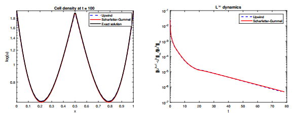
Left: Comparison of solutions of the Scharfetter-Gummel (red line) and upwind (blue, dashed line) schemes at time
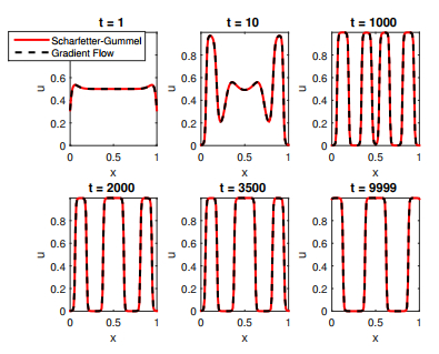
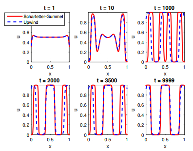
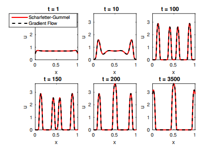
Evolution in time of solutions to (25) in the logistic case
Evolution in time of solutions to 25 in the logistic case
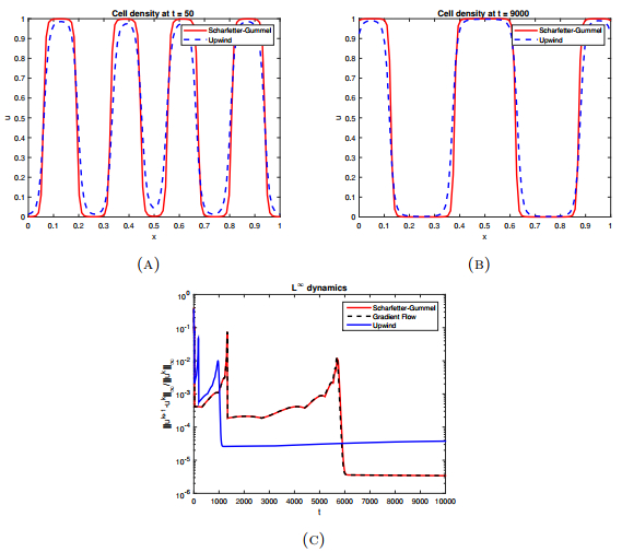
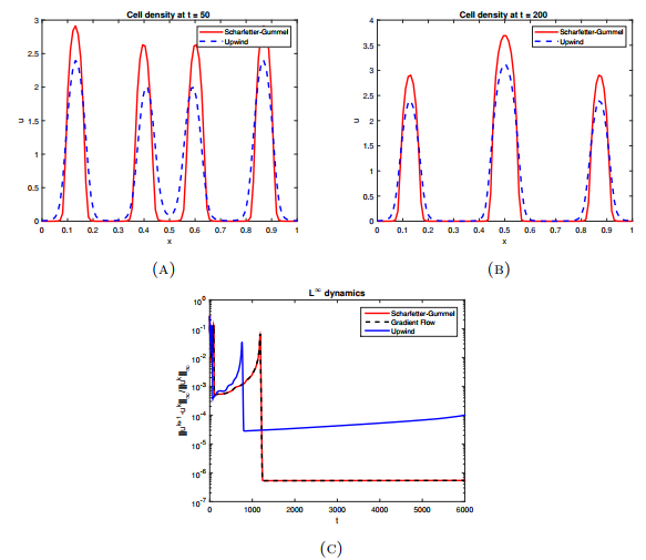
Stationary profiles and dynamics. (A), (B) Comparison of the stationary profiles of solutions to the Scharfetter-Gummel (red line) and the upwind (blue, dashed line) schemes at
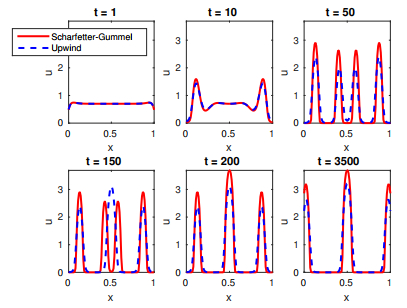
Evolution in time of solutions to 25 in the exponential case
Stationary profiles and dynamics. (A), (B)Comparison of the stationary profiles obtained with the Scharfetter-Gummel (red line) and the upwind scheme (blue, dashed line) at
Evolution in time of solutions to 25 in the exponential case


 DownLoad: