Visual perception of moving objects is integral to our day-to-day life, integrating visual spatial and temporal perception. Most research studies have focused on finding the brain regions activated during motion perception. However, an empirically validated general mathematical model is required to understand the modulation of the motion perception. Here, we develop a mathematical formulation of the modulation of the perception of a moving object due to a change in speed, under the formulation of the invariance of causality.
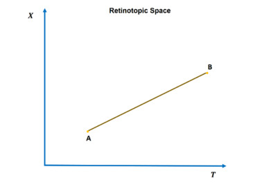
We formulated the perception of a moving object as the coordinate transformation from a retinotopic space onto perceptual space and derived a quantitative relationship between spatiotemporal coordinates. To validate our model, we undertook the analysis of two experiments: (i) the perceived length of the moving arc, and (ii) the perceived time while observing moving stimuli. We performed a magnetic resonance imaging (MRI) tractography investigation of subjects to demarcate the anatomical correlation of the modulation of the perception of moving objects.
Our theoretical model shows that the interaction between visual-spatial and temporal perception, during the perception of moving object is described by coupled linear equations; and experimental observations validate our model. We observed that cerebral area V5 may be an anatomical correlate for this interaction. The physiological basis of interaction is shown by a Lotka-Volterra system delineating interplay between acetylcholine and dopamine neurotransmitters, whose concentrations vary periodically with the orthogonal phase shift between them, occurring at the axodendritic synapse of complex cells at area V5.
Under the invariance of causality in the representation of events in retinotopic space and perceptual space, the speed modulates the perception of a moving object. This modulation may be due to variations of the tuning properties of complex cells at area V5 due to the dynamic interaction between acetylcholine and dopamine. Our analysis is the first significant study, to our knowledge, that establishes a mathematical linkage between motion perception and causality invariance.
Citation: Pratik Purohit, Prasun K. Roy. Interaction between spatial perception and temporal perception enables preservation of cause-effect relationship: Visual psychophysics and neuronal dynamics[J]. Mathematical Biosciences and Engineering, 2023, 20(5): 9101-9134. doi: 10.3934/mbe.2023400
Visual perception of moving objects is integral to our day-to-day life, integrating visual spatial and temporal perception. Most research studies have focused on finding the brain regions activated during motion perception. However, an empirically validated general mathematical model is required to understand the modulation of the motion perception. Here, we develop a mathematical formulation of the modulation of the perception of a moving object due to a change in speed, under the formulation of the invariance of causality.
We formulated the perception of a moving object as the coordinate transformation from a retinotopic space onto perceptual space and derived a quantitative relationship between spatiotemporal coordinates. To validate our model, we undertook the analysis of two experiments: (i) the perceived length of the moving arc, and (ii) the perceived time while observing moving stimuli. We performed a magnetic resonance imaging (MRI) tractography investigation of subjects to demarcate the anatomical correlation of the modulation of the perception of moving objects.
Our theoretical model shows that the interaction between visual-spatial and temporal perception, during the perception of moving object is described by coupled linear equations; and experimental observations validate our model. We observed that cerebral area V5 may be an anatomical correlate for this interaction. The physiological basis of interaction is shown by a Lotka-Volterra system delineating interplay between acetylcholine and dopamine neurotransmitters, whose concentrations vary periodically with the orthogonal phase shift between them, occurring at the axodendritic synapse of complex cells at area V5.
Under the invariance of causality in the representation of events in retinotopic space and perceptual space, the speed modulates the perception of a moving object. This modulation may be due to variations of the tuning properties of complex cells at area V5 due to the dynamic interaction between acetylcholine and dopamine. Our analysis is the first significant study, to our knowledge, that establishes a mathematical linkage between motion perception and causality invariance.

| [1] |
M. G. P. Rosa, Visual maps in the adult primate cerebral cortex: Some implications for brain development and evolution, Braz. J. Med. Biol. Res., 35 (2002), 1485–1498. https://doi.org/10.1590/S0100-879X2002001200008 doi: 10.1590/S0100-879X2002001200008

|
| [2] |
H. Strasburger, On the cortical mapping function-Visual space, cortical space, and crowding, Vision Res., 194 (2022), 107972. https://doi.org/10.1016/j.visres.2021.107972 doi: 10.1016/j.visres.2021.107972
|
| [3] |
E. L. Schwartz, Computational anatomy and functional architecture of striate cortex: A spatial mapping approach to perceptual coding, Vision Res., 20 (1980), 645–669. https://doi.org/10.1016/0042-6989(80)90090-5 doi: 10.1016/0042-6989(80)90090-5
|
| [4] |
C. Bordier, J. M. Hupé, M. Dojat, Quantitative evaluation of fMRI retinotopic maps, from V1 to V4, for cognitive experiments, Front. Hum. Neurosci., 9 (2015), 277. https://doi.org/10.3389/fnhum.2015.00277 doi: 10.3389/fnhum.2015.00277
|
| [5] |
J. Larsson, D. J. Heeger, Two retinotopic visual areas in human lateral occipital cortex, J. Neurosci., 26 (2006), 13128–13142. https://doi.org/10.1523/JNEUROSCI.1657-06.2006 doi: 10.1523/JNEUROSCI.1657-06.2006
|
| [6] |
D. M. van Es, W. van der Zwaag, T. Knapen, Topographic maps of visual space in the human cerebellum, Curr. Biol., 29 (2019), 1689–1694. https://doi.org/10.1016/j.cub.2019.04.012 doi: 10.1016/j.cub.2019.04.012
|
| [7] |
C. A. Olman, P. F. Van de Moortele, J. F. Schumacher, J. R. Guy, K. Uǧurbil, E. Yacoub, Retinotopic mapping with spin echo BOLD at 7T, Magn. Reson. Imaging, 28 (2010), 1258–1269. https://doi.org/10.1016/j.mri.2010.06.001 doi: 10.1016/j.mri.2010.06.001
|
| [8] |
B. A. Wandell, J. Winawer, Imaging retinotopic maps in the human brain, Vision Res., 51 (2011), 718–737. https://doi.org/10.1016/j.visres.2010.08.004 doi: 10.1016/j.visres.2010.08.004
|
| [9] |
A. C. Huk, D. Ress, D. J. Heeger, Neuronal basis of the motion aftereffect reconsidered, Neuron, 32 (2001), 161–172. https://doi.org/10.1016/S0896-6273(01)00452-4 doi: 10.1016/S0896-6273(01)00452-4
|
| [10] |
K. Grill-Spector, T. Kushnir, T. Hendler, S. Edelman, Y. Itzchak, R. Malach, A sequence of object-processing stages revealed by fMRI in the human occipital lobe, Hum. Brain Mapp., 6 (1998), 316–328. https://doi.org/10.1002/(SICI)1097-0193(1998)6:4<316::AID-HBM9>3.0.CO;2-6 doi: 10.1002/(SICI)1097-0193(1998)6:4<316::AID-HBM9>3.0.CO;2-6
|
| [11] |
S. Engel, X. Zhang, B. Wandell, Colour tuning in human visual cortex measured with functional magnetic resonance imaging, Nature, 388 (1997), 68–71. https://doi.org/10.1038/40398 doi: 10.1038/40398
|
| [12] |
R. Hartig, C. Battal, G. Chávez, A. Vedoveli, T. Steudel, E. Krampe, et al., Topographic mapping of the primate primary interoceptive cortex, Front. Neurosci., 11 (2017). https://doi.org/10.3389/conf.fnins.2017.94.00005 doi: 10.3389/conf.fnins.2017.94.00005
|
| [13] |
J. A. Bourne, M. G. P. Rosa, Hierarchical development of the primate visual cortex, as revealed by neurofilament immunoreactivity: Early maturation of the middle temporal area (MT), Cereb. Cortex, 16 (2006), 405–414. https://doi.org/10.1093/cercor/bhi119 doi: 10.1093/cercor/bhi119
|
| [14] |
S. Nishida, T. Kawabe, M. Sawayama, T. Fukiage, Motion perception: From detection to interpretation, Annu. Rev. Vis. Sci., 4 (2018), 501–523. https://doi.org/10.1146/annurev-vision-091517-034328 doi: 10.1146/annurev-vision-091517-034328
|
| [15] |
T. D. Albright, G. R. Stoner, Visual motion perception, Proc. Natl. Acad. Sci. U. S. A., 92 (1995), 2433–2440. https://doi.org/10.1073/pnas.92.7.2433 doi: 10.1073/pnas.92.7.2433
|
| [16] |
A. M. Derrington, H. A. Allen, L. S. Delicato, Visual mechanisms of motion analysis and motion perception, Annu. Rev. Psychol., 55 (2004), 181–205. https://doi.org/10.1146/annurev.psych.55.090902.141903 doi: 10.1146/annurev.psych.55.090902.141903
|
| [17] |
J. D. Herrington, S. Baron-Cohen, S. J. Wheelwright, K. D. Singh, E. T. Bullmore, M. Brammer, et al., The role of MT+/V5 during biological motion perception in Asperger Syndrome: An fMRI study, Res. Autism Spectr. Disord., 1 (2007), 14–27. https://doi.org/10.1016/j.rasd.2006.07.002 doi: 10.1016/j.rasd.2006.07.002
|
| [18] |
A. Antal, M. A. Nitsche, W. Kruse, T. Z. Kincses, K. P. Hoffmann, W. Paulus, Direct current stimulation over V5 enhances visuomotor coordination by improving motion perception in humans, J. Cogn. Neurosci., 16 (2004), 521–527. https://doi.org/10.1162/089892904323057263 doi: 10.1162/089892904323057263
|
| [19] |
R. Laycock, D. P. Crewther, P. B. Fitzgerald, S. G. Crewther, Evidence for fast signals and later processing in human V1/V2 and V5/MT+: A TMS study of motion perception, J. Neurophysiol., 98 (2007), 1253–1262. https://doi.org/10.1152/jn.00416.2007 doi: 10.1152/jn.00416.2007
|
| [20] |
D. Tadin, J. Silvanto, A. Pascual-Leone, L. Battelli, Improved motion perception and impaired spatial suppression following disruption of cortical area MT/V5, J. Neurosci., 31 (2011), 1279–1283. https://doi.org/10.1523/JNEUROSCI.4121-10.2011 doi: 10.1523/JNEUROSCI.4121-10.2011
|
| [21] |
J. P. H. van Santen, G. Sperling, Elaborated Reichardt detectors, J. Opt. Soc. Am. A, 2 (1985), 300. https://doi.org/10.1364/josaa.2.000300 doi: 10.1364/josaa.2.000300
|
| [22] |
E. H. Adelson, J. R. Bergen, Spatiotemporal energy models for the perception of motion, J. Opt. Soc. Am. A, 2 (1985), 284. https://doi.org/10.1364/josaa.2.000284 doi: 10.1364/josaa.2.000284
|
| [23] |
M. Mashour, The information basis in the perception of velocity, Acta Psychol. (Amst)., 48 (1981), 69–78. https://doi.org/10.1016/0001-6918(81)90049-4 doi: 10.1016/0001-6918(81)90049-4
|
| [24] |
D. Algom, L. Cohen-Raz, Visual velocity input-output functions: The integration of distance and duration onto subjective velocity, J. Exp. Psychol. Hum. Percept. Perform., 10 (1984), 486–501. https://doi.org/10.1037/0096-1523.10.4.486 doi: 10.1037/0096-1523.10.4.486
|
| [25] |
D. J. Hagler, M. I. Sereno, Spatial maps in frontal and prefrontal cortex, Neuroimage, 29 (2006), 567–577. https://doi.org/10.1016/j.neuroimage.2005.08.058 doi: 10.1016/j.neuroimage.2005.08.058
|
| [26] |
S. D. Slotnick, S. A. Klein, T. Carney, E.E. Sutter, Electrophysiological estimate of human cortical magnification, Clin. Neurophysiol., 112 (2001), 1349–1356. https://doi.org/10.1016/S1388-2457(01)00561-2 doi: 10.1016/S1388-2457(01)00561-2
|
| [27] |
J. Swearer, Visual Angle, Encycl. Clin. Neuropsychol., (2011), 2626–2627. https://doi.org/10.1007/978-0-387-79948-3_1411 doi: 10.1007/978-0-387-79948-3_1411
|
| [28] |
A. Cowey, E. T. Rolls, Human cortical magnification factor and its relation to visual acuity, Exp. Brain Res., 21 (1974), 447–454. https://doi.org/10.1007/BF00237163 doi: 10.1007/BF00237163
|
| [29] |
H. L. Ansbacher, Distortion in the perception of real movement, J. Exp. Psychol., 34 (1944), 1–23. https://doi.org/10.1037/h0061686 doi: 10.1037/h0061686
|
| [30] |
S. Kaneko, I. Murakami, Perceived duration of visual motion increases with speed, J. Vis., 9 (2009), 1–12. https://doi.org/10.1167/9.7.14 doi: 10.1167/9.7.14
|
| [31] |
K. R. Sitek, O. F. Gulban, E. Calabrese, G. A. Johnson, A. Lage-Castellanos, M. Moerel, et al., Mapping the human subcortical auditory system using histology, postmortem MRI and in vivo MRI at 7T, Elife, 8 (2019), 1–36. https://doi.org/10.7554/eLife.48932 doi: 10.7554/eLife.48932
|
| [32] |
P. J. Basser, J. Mattiello, D. Lebihan, Estimation of the effective self-diffusion tensor from the NMR spin echo, J. Magn. Reson. Ser. B, 103 (1994), 247–254. https://doi.org/10.1006/jmrb.1994.1037 doi: 10.1006/jmrb.1994.1037
|
| [33] |
L. Fan, H. Li, J. Zhuo, Y. Zhang, J. Wang, L. Chen, et al., The human brainnetome atlas: A new brain atlas based on connectional architecture, Cereb. Cortex, 26 (2016), 3508–3526. https://doi.org/10.1093/cercor/bhw157 doi: 10.1093/cercor/bhw157
|
| [34] |
R. O. Duncan, G. M. Boynton, Cortical magnification within human primary visual cortex correlates with acuity thresholds, Neuron, 38 (2003), 659–671. https://doi.org/10.1016/S0896-6273(03)00265-4 doi: 10.1016/S0896-6273(03)00265-4
|
| [35] |
J. C. Horton, W. F. Hoyt, The representation of the visual field in human striate cortex: A revision of the classic Holmes map, Arch. Ophthalmol., 109 (1991), 816–824. https://doi.org/10.1001/archopht.1991.01080060080030 doi: 10.1001/archopht.1991.01080060080030
|
| [36] |
J. Rovamo, V. Virsu, An estimation and application of the human cortical magnification factor, Exp. Brain Res., 37 (1979), 495–510. https://doi.org/10.1007/BF00236819 doi: 10.1007/BF00236819
|
| [37] |
M. M. Schira, A. R. Wade, C. W. Tyler, Two-dimensional mapping of the central and parafoveal visual field to human visual cortex, J. Neurophysiol., 97 (2007), 4284–4295. https://doi.org/10.1152/jn.00972.2006 doi: 10.1152/jn.00972.2006
|
| [38] | D. J. Tolhurst, L. Ling, Magnification factors and the organization of the human striate cortex, Hum. Neurobiol., 6 (1988), 247–254. |
| [39] | J. Mate, A. C. Pires, G. Campoy, S. Estaún, Estimating the duration of visual stimuli in motion environments., Psicológica, 30 (2009), 287–300. |
| [40] |
H. Karşilar, Y. D. Kisa, F. Balci, Dilation and constriction of subjective time based on observed walking speed, Front. Psychol., 9 (2018), 2565. https://doi.org/10.3389/fpsyg.2018.02565 doi: 10.3389/fpsyg.2018.02565
|
| [41] | S. W. brown, Time, change, and motion: The effects of stimulus movement on temporal perception, Percept. Psychophys., 57 (1995), 105–116. https://doi.org/10.3758/BF03211853 |
| [42] |
A. Petzold, E. Pitz, The historical origin of the pulfrich effect: A serendipitous astronomic observation at the border of the Milky Way, Neuro-Ophthalmology, 33 (2009), 39–46. https://doi.org/10.1080/01658100802590829 doi: 10.1080/01658100802590829
|
| [43] |
J. A. Wilson, S. M. Anstis, Visual delay as a function of luminance, Am. J. Psychol., 82 (1969), 350–358. https://doi.org/10.2307/1420750 doi: 10.2307/1420750
|
| [44] |
A. Reynaud, R. F. Hess, Interocular contrast difference drives illusory 3D percept, Sci. Rep., 7 (2017), 1–6. https://doi.org/10.1038/s41598-017-06151-w doi: 10.1038/s41598-017-06151-w
|
| [45] |
N. Qian, R. A. Andersen, A physiological model for motion-stereo integration and a unified explanation of Pulfrich-like phenomena, Vision Res., 37 (1997), 1683–1698. https://doi.org/10.1016/S0042-6989(96)00164-2 doi: 10.1016/S0042-6989(96)00164-2
|
| [46] |
A. Anzai, I. Ohzawa, R. D. Freeman, Joint-encoding of motion and depth by visual cortical neurons: Neural basis of the Pulfrich effect, Nat. Neurosci., 4 (2001), 513–518. https://doi.org/10.1038/87462 doi: 10.1038/87462
|
| [47] |
A. A. L. D'Alfonso, J. Van Honk, D. J. L. G. Schutter, A. R. Caffé, A. Postma, E. H. F. De Haan, Spatial and temporal characteristics of visual motion perception involving V5 visual cortex, Neurol. Res., 24 (2002), 266–270. https://doi.org/10.1179/016164102101199891 doi: 10.1179/016164102101199891
|
| [48] |
G. Beckers, S. Zeki, The consequences of inactivating areas V1 and V5 on visual motion perception, Brain, 118 (1995), 49–60. https://doi.org/10.1093/brain/118.1.49 doi: 10.1093/brain/118.1.49
|
| [49] |
R. Laycock, D. P. Crewther, P. B. Fitzgerald, S. G. Crewther, Evidence for fast signals and later processing in human V1/V2 and V5/MT+: A TMS study of motion perception, J. Neurophysiol., 98 (2007), 1253–1262. https://doi.org/10.1152/jn.00416.2007 doi: 10.1152/jn.00416.2007
|
| [50] |
K. Spang, M. Morgan, Cortical correlates of stereoscopic depth produced by temporal delay, J. Vis., 8 (2008), 1–12. https://doi.org/10.1167/8.9.10 doi: 10.1167/8.9.10
|
| [51] |
R. A. Andersen, G. K. Essick, R. M. Siegel, Encoding of spatial location by posterior parietal neurons, Science, 230 (1985), 456–458. https://doi.org/10.1126/science.4048942 doi: 10.1126/science.4048942
|
| [52] |
A. M. Ferrandez, L. Hugueville, S. Lehéricy, J. B. Poline, C. Marsault, V. Pouthas, Basal ganglia and supplementary motor area subtend duration perception: An fMRI study, Neuroimage, 19 (2003), 1532–1544. https://doi.org/10.1016/S1053-8119(03)00159-9 doi: 10.1016/S1053-8119(03)00159-9
|
| [53] |
D. L. Harrington, K. Y. Haaland, R. T. Knight, Cortical networks underlying mechanisms of time perception, J. Neurosci., 18 (1998), 1085–1095. https://doi.org/10.1523/jneurosci.18-03-01085.1998 doi: 10.1523/jneurosci.18-03-01085.1998
|
| [54] |
R. B. Ivry, R. M. C. Spencer, The neural representation of time, Curr. Opin. Neurobiol., 14 (2004), 225–232. https://doi.org/10.1016/j.conb.2004.03.013 doi: 10.1016/j.conb.2004.03.013
|
| [55] |
P. Janssen, M. N. Shadlen, A representation of the hazard rate of elapsed time in macaque area LIP, Nat. Neurosci., 8 (2005), 234–241. https://doi.org/10.1038/nn1386 doi: 10.1038/nn1386
|
| [56] |
M. Jazayeri, M. N. Shadlen, A neural mechanism for sensing and reproducing a time interval, Curr. Biol., 25 (2015), 2599–2609. https://doi.org/10.1016/j.cub.2015.08.038 doi: 10.1016/j.cub.2015.08.038
|
| [57] |
C. S. Konen, S. Kastner, Representation of eye movements and stimulus motion in topographically organized areas of human posterior parietal cortex, J. Neurosci., 28 (2008), 8361–8375. https://doi.org/10.1523/JNEUROSCI.1930-08.2008 doi: 10.1523/JNEUROSCI.1930-08.2008
|
| [58] |
M. I. Leon, M. N. Shadlen, Representation of time by neurons in the posterior parietal cortex of the macaque, Neuron, 38 (2003), 317–327. https://doi.org/https://doi.org/10.1016/S0896-6273(03)00185-5 doi: 10.1016/S0896-6273(03)00185-5
|
| [59] |
P. A. Lewis, R. C. Miall, Distinct systems for automatic and cognitively controlled time measurement: Evidence from neuroimaging, Curr. Opin. Neurobiol., 13 (2003), 250–255. https://doi.org/10.1016/S0959-4388(03)00036-9 doi: 10.1016/S0959-4388(03)00036-9
|
| [60] |
H. Onoe, M. Komori, K. Onoe, H. Takechi, H. Tsukada, Y. Watanabe, Cortical networks recruited for time perception: A monkey positron emission tomography (PET) study, Neuroimage, 13 (2001), 37–45. https://doi.org/10.1006/nimg.2000.0670 doi: 10.1006/nimg.2000.0670
|
| [61] | F. Protopapa, M. J. Hayashi, S. Kulashekhar, W. Van Der Zwaag, G. Battistella, M. M. Murray, et al., Chronotopic maps in human supplementary motor area, 17 (2019), e3000026. https://doi.org/10.1371/journal.pbio.3000026 |
| [62] |
H. Sakata, M. Kusunoki, Organization of space perception: neural representation of three-dimensional space in the posterior parietal cortex, Curr. Opin. Neurobiol., 2 (1992), 170–174. https://doi.org/10.1016/0959-4388(92)90007-8 doi: 10.1016/0959-4388(92)90007-8
|
| [63] |
J. G. Mikhael, S. J. Gershman, Adapting the flow of time with dopamine, J. Neurophysiol., 121 (2019), 1748–1760. https://doi.org/10.1152/jn.00817.2018 doi: 10.1152/jn.00817.2018
|
| [64] |
T. Liu, P. Hu, R. Cao, X. Ye, Y. Tian, X. Chen, et al., Dopaminergic modulation of biological motion perception in patients with Parkinson's disease, Sci. Rep., 7 (2017), 1–9. https://doi.org/10.1038/s41598-017-10463-2 doi: 10.1038/s41598-017-10463-2
|
| [65] |
C. Gratton, S. Yousef, E. Aarts, D. L. Wallace, M. D'Esposito, M. A. Silver, Cholinergic, but not dopaminergic or noradrenergic, enhancement sharpens visual spatial perception in humans, J. Neurosci., 37 (2017), 4405–4415. https://doi.org/10.1523/JNEUROSCI.2405-16.2017 doi: 10.1523/JNEUROSCI.2405-16.2017
|
| [66] |
S. Threlfell, M. A. Clements, T. Khodai, I. S. Pienaar, R. Exley, J. Wess, et al., Striatal muscarinic receptors promote activity dependence of dopamine transmission via distinct receptor subtypes on cholinergic interneurons in ventral versus dorsal striatum, J. Neurosci., 30 (2010), 3398–3408. https://doi.org/10.1523/JNEUROSCI.5620-09.2010 doi: 10.1523/JNEUROSCI.5620-09.2010
|
| [67] |
S. Threlfell, T. Lalic, N. J. Platt, K. A. Jennings, K. Deisseroth, S. J. Cragg, Striatal dopamine release is triggered by synchronized activity in cholinergic interneurons, Neuron, 75 (2012), 58–64. https://doi.org/10.1016/j.neuron.2012.04.038 doi: 10.1016/j.neuron.2012.04.038
|
| [68] |
E. D. Abercrombie, P. DeBoer, Substantia nigra D1 receptors and stimulation of striatal cholinergic interneurons by dopamine: A proposed circuit mechanism, J. Neurosci., 17 (1997), 8498–8505. https://doi.org/10.1523/jneurosci.17-21-08498.1997 doi: 10.1523/jneurosci.17-21-08498.1997
|
| [69] |
B. Di Cara, F. Panayi, A. Gobert, A. Dekeyne, D. Sicard, L. De Groote, et al., Activation of dopamine D1 receptors enhances cholinergic transmission and social cognition: A parallel dialysis and behavioural study in rats, Int. J. Neuropsychopharmacol., 10 (2007), 383–399. https://doi.org/10.1017/S1461145706007103 doi: 10.1017/S1461145706007103
|
| [70] |
A. Imperato, M. C. Obinu, G. L. Gessa, Stimulation of both dopamine D1 and D2 receptors facilitates in vivo acetylcholine release in the hippocampus, Brain Res., 618 (1993), 341–345. https://doi.org/10.1016/0006-8993(93)91288-4 doi: 10.1016/0006-8993(93)91288-4
|
| [71] |
A. Martorana, F. Mori, Z. Esposito, H. Kusayanagi, F. Monteleone, C. Codecà, et al., Dopamine modulates cholinergic cortical excitability in Alzheimer's disease patients, Neuropsychopharmacology, 34 (2009), 2323–2328. https://doi.org/10.1038/npp.2009.60 doi: 10.1038/npp.2009.60
|
| [72] |
M. S. Lidow, P. S. Goldman-Rakic, D. W. Gallager, P. Rakic, Distribution of dopaminergic receptors in the primate cerebral cortex: Quantitative autoradiographic analysis using 3H.raclopride, 3H.spiperone and 3H.SCH23390, Neuroscience, 40 (1991), 657–671. https://doi.org/10.1016/0306-4522(91)90003-7 doi: 10.1016/0306-4522(91)90003-7
|
| [73] |
A. Mueller, R. M. Krock, S. Shepard, T. Moore, Dopamine receptor expression among local and visual cortex-projecting frontal eye field neurons, Cereb. Cortex, 30 (2020), 148–164. https://doi.org/10.1093/cercor/bhz078 doi: 10.1093/cercor/bhz078
|
| [74] |
K. Zilles, N. Palomero-Gallagher, Multiple transmitter receptors in regions and layers of the human cerebral cortex, Front. Neuroanat., 11 (2017), 1–26. https://doi.org/10.3389/fnana.2017.00078 doi: 10.3389/fnana.2017.00078
|
| [75] |
J. McLean, L. A. Palmer, Contribution of linear spatiotemporal receptive field structure to velocity selectivity of simple cells in area 17 of cat, Vision Res., 29 (1989), 675–679. https://doi.org/10.1016/0042-6989(89)90029-1 doi: 10.1016/0042-6989(89)90029-1
|
| [76] |
A. S. Pawar, S. Gepshtein, S. Savel'ev, T. D. Albright, Mechanisms of spatiotemporal selectivity in cortical area MT, Neuron, 101 (2019), 514–527. https://doi.org/10.1016/j.neuron.2018.12.002 doi: 10.1016/j.neuron.2018.12.002
|
| [77] |
N. J. Priebe, C. R. Cassanello, S. G. Lisberger, The neural representation of speed in macaque area MT/V5, J. Neurosci., 23 (2003), 5650–5661. https://doi.org/10.1523/jneurosci.23-13-05650.2003 doi: 10.1523/jneurosci.23-13-05650.2003
|
| [78] |
D. Giaschi, A. Zwicker, S. A. Young, B. Bjornson, The role of cortical area V5/MT+ in speed-tuned directional anisotropies in global motion perception, Vision Res., 47 (2007), 887–898. https://doi.org/10.1016/j.visres.2006.12.017 doi: 10.1016/j.visres.2006.12.017
|
| [79] |
J. A. Perrone, A. Thiele, A model of speed tuning in MT neurons, Vision Res., 42 (2002), 1035–1051. https://doi.org/10.1016/S0042-6989(02)00029-9 doi: 10.1016/S0042-6989(02)00029-9
|
| [80] |
D. C. Penn, K. J. Holyoak, D. J. Povinelli, Darwin's mistake: Explaining the discontinuity between human and nonhuman minds, Behav. Brain Sci., 31 (2008), 109–178. https://doi.org/10.1017/S0140525X08003543 doi: 10.1017/S0140525X08003543
|
| [81] |
M. Stuart-Fox, The origins of causal cognition in early hominins, Biol. Philos., 30 (2015), 247–266. https://doi.org/10.1007/s10539-014-9462-y doi: 10.1007/s10539-014-9462-y
|
| [82] |
J. A. Perrone, A. Thiele, Speed skills: measuring the visual speed analyzing properties of primate MT neurons, Nat. Neurosci., 4 (2001), 526–532. https://doi.org/10.1038/87480 doi: 10.1038/87480
|
| [83] |
G. Riddoch, Dissociation of visual perceptions due to occipital injuries, with especial reference to appreciation of movement, Brain, 40 (1917), 15–57. https://doi.org/10.1093/brain/40.1.15 doi: 10.1093/brain/40.1.15
|
| [84] |
S. Zeki, D.H. Ffytche, The Riddoch syndrome: Insights into the neurobiology of conscious vision, Brain, 121 (1998), 25–45. https://doi.org/10.1093/brain/121.1.25 doi: 10.1093/brain/121.1.25
|
| [85] |
T. Amemiya, B. Beck, V. Walsh, H. Gomi, P. Haggard, Visual area V5/hMT+ contributes to perception of tactile motion direction: A TMS study, Sci. Rep., 7 (2017), 1–7. https://doi.org/10.1038/srep40937 doi: 10.1038/srep40937
|
| [86] |
K. Krug, A common neuronal code for perceptual processes in visual cortex? Comparing choice and attentional correlates in V5/MT, Philos. Trans. R. Soc. B Biol. Sci., 359 (2004), 929–941. https://doi.org/10.1098/rstb.2003.1415 doi: 10.1098/rstb.2003.1415
|
| [87] |
C. Poirier, O. Collignon, A. G. DeVolder, L. Renier, A. Vanlierde, D. Tranduy, et al., Specific activation of the V5 brain area by auditory motion processing: An fMRI study, Cogn. Brain Res., 25 (2005), 650–658. https://doi.org/10.1016/j.cogbrainres.2005.08.015 doi: 10.1016/j.cogbrainres.2005.08.015
|
| [88] |
S. Zeki, Area V5—a microcosm of the visual brain, Front. Integr. Neurosci., 9 (2015), 1–18. https://doi.org/10.3389/fnint.2015.00021 doi: 10.3389/fnint.2015.00021
|
| [89] |
J. Kim, D. Norton, R. McBain, D. Ongur, Y. Chen, Deficient biological motion perception in schizophrenia: Results from a motion noise paradigm, Front. Psychol., 4 (2013), 391. https://doi.org/10.3389/fpsyg.2013.00391 doi: 10.3389/fpsyg.2013.00391
|
| [90] |
Y. Chen, Abnormal visual motion processing in schizophrenia: A review of research progress, Schizophr. Bull., 37 (2011), 709–715. https://doi.org/10.1093/schbul/sbr020 doi: 10.1093/schbul/sbr020
|
| [91] |
J. D. Golomb, J. R. B. McDavitt, B. M. Ruf, J. I. Chen, A. Saricicek, K. H. Maloney, et al., Enhanced visual motion perception in major depressive disorder, J. Neurosci., 29 (2009), 9072–9077. https://doi.org/10.1523/JNEUROSCI.1003-09.2009 doi: 10.1523/JNEUROSCI.1003-09.2009
|
| [92] |
L. Richard, D. Charbonneau, An introduction to E-Prime, Tutor. Quant. Methods Psychol., 5 (2009), 68–76. https://doi.org/10.20982/tqmp.05.2.p068 doi: 10.20982/tqmp.05.2.p068
|
| [93] |
J. W. Peirce, PsychoPy-Psychophysics software in Python, J. Neurosci. Methods, 162 (2007), 8–13. https://doi.org/10.1016/j.jneumeth.2006.11.017 doi: 10.1016/j.jneumeth.2006.11.017
|
| [94] |
J. Ceccarini, H. Liu, K. Van Laere, E. D. Morris, C. Y. Sander, Methods for quantifying neurotransmitter dynamics in the living brain with PET imaging, Front. Physiol., 11 (2020), 792. https://doi.org/10.3389/fphys.2020.00792 doi: 10.3389/fphys.2020.00792
|
| [95] |
E. J. Novotny, R. K. Fulbright, P. L. Pearl, K. M. Gibson, D. L. Rothman, Magnetic resonance spectroscopy of neurotransmitters in human brain, Ann. Neurol., 54 (2003), S25–S31. https://doi.org/10.1002/ana.10697 doi: 10.1002/ana.10697
|
| [96] |
A. Routier, N. Burgos, M. Díaz, M. Bacci, S. Bottani, O. El-Rifai, et al., Clinica: An open-source software platform for reproducible clinical neuroscience studies, Front. Neuroinform., 15 (2021), 39. https://doi.org/10.3389/fninf.2021.689675 doi: 10.3389/fninf.2021.689675
|
| [97] |
W. T. Clarke, C. J. Stagg, S. Jbabdi, FSL-MRS: An end-to-end spectroscopy analysis package, Magn. Reson. Med., 85 (2021), 2950–2964. https://doi.org/10.1002/mrm.28630 doi: 10.1002/mrm.28630
|
 mbe-20-05-400-supplementary.pdf mbe-20-05-400-supplementary.pdf |
 |


Figures(15) / Tables(1)

Pratik Purohit, Prasun K. Roy. Interaction between spatial perception and temporal perception enables preservation of cause-effect relationship: Visual psychophysics and neuronal dynamics[J]. Mathematical Biosciences and Engineering, 2023, 20(5): 9101-9134. doi: 10.3934/mbe.2023400


 DownLoad: