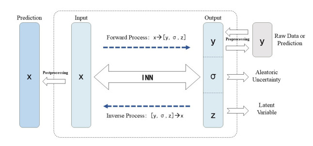
Invertible neural network (INN) is a promising tool for inverse design optimization. While generating forward predictions from given inputs to the system response, INN enables the inverse process without much extra cost. The inverse process of INN predicts the possible input parameters for the specified system response qualitatively. For the purpose of design space exploration and reasoning for critical engineering systems, accurate predictions from the inverse process are required. Moreover, INN predictions lack effective uncertainty quantification for regression tasks, which increases the challenges of decision making. This paper proposes the probabilistic invertible neural network (P-INN): the epistemic uncertainty and aleatoric uncertainty are integrated with INN. A new loss function is formulated to guide the training process with enhancement in the inverse process accuracy. Numerical evaluations have shown that the proposed P-INN has noticeable improvement on the inverse process accuracy and the prediction uncertainty is reliable.
Citation: Yiming Zhang, Zhiwei Pan, Shuyou Zhang, Na Qiu. Probabilistic invertible neural network for inverse design space exploration and reasoning[J]. Electronic Research Archive, 2023, 31(2): 860-881. doi: 10.3934/era.2023043
Invertible neural network (INN) is a promising tool for inverse design optimization. While generating forward predictions from given inputs to the system response, INN enables the inverse process without much extra cost. The inverse process of INN predicts the possible input parameters for the specified system response qualitatively. For the purpose of design space exploration and reasoning for critical engineering systems, accurate predictions from the inverse process are required. Moreover, INN predictions lack effective uncertainty quantification for regression tasks, which increases the challenges of decision making. This paper proposes the probabilistic invertible neural network (P-INN): the epistemic uncertainty and aleatoric uncertainty are integrated with INN. A new loss function is formulated to guide the training process with enhancement in the inverse process accuracy. Numerical evaluations have shown that the proposed P-INN has noticeable improvement on the inverse process accuracy and the prediction uncertainty is reliable.

| [1] |
S. Ghosh, G. A. Padmanabha, C. Peng, V. Andreoli, S. Atkinson, P. Pandita, et al., Inverse aerodynamic design of Gas turbine blades using probabilistic machine learning, J. Mech. Des., 144 (2022), 021706. https://doi.org/10.1115/1.4052301 doi: 10.1115/1.4052301

|
| [2] |
S. Obayashi, S Takanashi, Genetic optimization of target pressure distributions for inverse design methods, AIAA J., 34 (1996), 881–886. https://doi.org/10.2514/3.13163 doi: 10.2514/3.13163
|
| [3] |
P. Boselli, M. Zangeneh, An inverse design based methodology for rapid 3D multi-objective/multidisciplinary optimization of axial turbines, ASME J. Turbomach., 7 (2011), 1459–1468. https://doi.org/10.1115/GT2011-46729 doi: 10.1115/GT2011-46729
|
| [4] |
A. Nickless, P. J. Rayner, B. Erni, R. J. Scholes, Comparison of the genetic algorithm and incremental optimisation routines for a Bayesian inverse modelling based network design, Inverse Probl., 34 (2018), 055006. https://doi.org/10.1088/1361-6420/aab46c doi: 10.1088/1361-6420/aab46c
|
| [5] |
B. Hofmeister, M. Bruns, R. Rolfes, Finite element model updating using deterministic optimisation: a global pattern search approach, Eng. Struct., 195 (2019), 373–381. https://doi.org/10.1016/j.engstruct.2019.05.047 doi: 10.1016/j.engstruct.2019.05.047
|
| [6] | S. S. Kadre, V. K. Tripathi, Advanced surrogate models for design optimization, Int. J. Eng. Sci., 9 (2016), 66–73. |
| [7] | C. P. Robert, G. Casella, Monte Carlo Statistical Methods, Springer New York, 2004. https://doi.org/10.1007/978-1-4757-4145-2 |
| [8] | J. Jiang, Large Sample Techniques for Statistics, Cham, Springer International Publishing, 2022. https://doi.org/10.1007/978-3-030-91695-4 |
| [9] |
D. M. Blei, A. Kucukelbir, J. D. McAuliffe, Variational inference: a review for statisticians, J. Am. Stat. Assoc., 112 (2017), 859–877. https://doi.org/10.1080/01621459.2017.1285773 doi: 10.1080/01621459.2017.1285773
|
| [10] |
L. Wu, W. Ji, S. M. AbouRizk, Bayesian inference with markov chain monte carlo–based numerical approach for input model updating, J. Comput. Civ. Eng., 34 (2020), 04019043. https://doi.org/10.1061/(ASCE)CP.1943-5487.0000862 doi: 10.1061/(ASCE)CP.1943-5487.0000862
|
| [11] |
J. J. Xu, W. G. Chen, C. Demartino, T. Y. Xie, Y. Yu, C. F. Fang, et al., A Bayesian model updating approach applied to mechanical properties of recycled aggregate concrete under uniaxial or triaxial compression, Constr. Build. Mater., 301 (2021), 124274. https://doi.org/10.1016/j.conbuildmat.2021.124274 doi: 10.1016/j.conbuildmat.2021.124274
|
| [12] |
Y. Yin, W. Yin, P. Meng, H. Liu, On a hybrid approach for recovering multiple obstacles, Commun. Comput. Phys., 31 (2022), 869–892. https://doi.org/10.4208/cicp.OA-2021-0124 doi: 10.4208/cicp.OA-2021-0124
|
| [13] | N. C. Laurenciu, S. D. Cotofana, Probability density function based reliability evaluation of large-scale ICs, in Proceedings of the 2014 IEEE/ACM International Symposium on Nanoscale Architectures, (2014), 157–162. https://doi.org/10.1145/2770287.2770326 |
| [14] |
V. Raj, S. Kalyani, Design of communication systems using deep learning: a variational inference perspective, IEEE Trans. Cognit. Commun. Networking, 6 (2020), 1320–1334. https://doi.org/10.1109/TCCN.2020.2985371 doi: 10.1109/TCCN.2020.2985371
|
| [15] |
H. Liu, On local and global structures of transmission eigenfunctions and beyond, J. Inverse Ill-Posed Probl., 30 (2020), 287–305. https://doi.org/10.1515/jiip-2020-0099 doi: 10.1515/jiip-2020-0099
|
| [16] |
Y. Gao, H. Liu, X. Wang, K. Zhang, On an artificial neural network for inverse scattering problems, J. Comput. Phys., 448 (2022), 110771. https://doi.org/10.1016/j.jcp.2021.110771 doi: 10.1016/j.jcp.2021.110771
|
| [17] |
W. Yin, W. Yang, H. Liu, A neural network scheme for recovering scattering obstacles with limited phaseless far-field data, J. Comput. Phys., 417 (2020), 109594. https://doi.org/10.1016/j.jcp.2020.109594 doi: 10.1016/j.jcp.2020.109594
|
| [18] |
P. Zhang, P. Meng, W. Yin, H. Liu, A neural network method for time-dependent inverse source problem with limited-aperture data, J. Comput. Appl. Math., 421 (2023), 114842. https://doi.org/10.1016/j.cam.2022.114842 doi: 10.1016/j.cam.2022.114842
|
| [19] |
Y. Lu, Z. Tu, A two-level neural network approach for dynamic FE model updating including damping, J. Sound Vib., 275 (2004), 931–952. https://doi.org/10.1016/S0022-460X(03)00796-X doi: 10.1016/S0022-460X(03)00796-X
|
| [20] | H. Sung, S. Chang, M. Cho, Reduction method based structural model updating method via neural networks, 2020. https://doi.org/10.2514/6.2020-1445 |
| [21] |
H. Sung, S. Chang, M. Cho, Efficient model updating method for system identification using a convolutional neural network, AIAAJ, 59 (2021), 3480–3489. https://doi.org/10.2514/1.J059964 doi: 10.2514/1.J059964
|
| [22] |
T. Yin, H. Zhu, An efficient algorithm for architecture design of Bayesian neural network in structural model updating, Comput.-Aided Civ. Infrastruct. Eng., 35 (2020), 354–372. https://doi.org/10.1111/mice.12492 doi: 10.1111/mice.12492
|
| [23] | D. P. Kingma, T. Salimans, M. Welling, Variational dropout and the local reparameterization trick, in Advances in Neural Information Processing Systems, 28 (2015). Available from: https://proceedings.neurips.cc/paper/2015/file/bc7316929fe1545bf0b98d114ee3ecb8-Paper.pdf. |
| [24] | A. Kendall, Y. Gal, What uncertainties do we need in bayesian deep learning for computer vision? in Advances in Neural Information Processing Systems, 30 (2017). Available from: https://proceedings.neurips.cc/paper/2017/file/2650d6089a6d640c5e85b2b88265dc2b-Paper.pdf. |
| [25] |
E. Yilmaz, B. German, Conditional generative adversarial network framework for airfoil inverse design, AIAA, 2020 (2020). https://doi.org/10.2514/6.2020-3185 doi: 10.2514/6.2020-3185
|
| [26] | J. A. Hodge, K. V. Mishra, A. I. Zaghloul, Joint multi-layer GAN-based design of tensorial RF metasurfaces, in 2019 IEEE 29th International Workshop on Machine Learning for Signal Processing (MLSP), (2019), 1–6. https://doi.org/10.1109/MLSP.2019.8918860 |
| [27] | A. H. Nobari, W. Chen, F. Ahmed, PcDGAN: A continuous conditional diverse generative adversarial network for inverse design, preprint, arXiv: 2106.03620. |
| [28] | A. H. Nobari, W. Chen, F. Ahmed, Range-GAN: Range-constrained generative adversarial network for conditioned design synthesis, in Proceedings of the ASME 2021 International Design Engineering Technical Conferences and Computers and Information in Engineering Conference, 3B (2021), V03BT03A039. https://doi.org/10.1115/DETC2021-69963 |
| [29] | L. Ardizzone, J. Kruse, S. Wirkert, D. Rahner, E. W. Pellegrini, R. S. Klessen, et al., Analyzing inverse problems with invertible neural networks, preprint, arXiv: 1808.04730. |
| [30] | L. Dinh, D. Krueger, Y. Bengio, NICE: Non-linear independent components estimation, preprint, arXiv: 1410.8516. |
| [31] | L. Dinh, J. Sohl-Dickstein, S. Bengio, Density estimation using real NVP, preprint, arXiv: 1605.08803. |
| [32] | Z. Guan, J. Jing, X. Deng, M. Xu, L. Jiang, Z. Zhang, et al., DeepMIH: Deep invertible network for multiple image hiding, IEEE Trans. Pattern Anal. Mach. Intell., 2022 (2022). https://doi.org/10.1109/TPAMI.2022.3141725 |
| [33] | Y. Liu, Z. Qin, S. Anwar, P. Ji, D. Kim, S. Caldwell, et al., Invertible denoising network: a light solution for real noise removal, in 2021 IEEE/CVF Conference on Computer Vision and Pattern Recognition (CVPR), (2021), 13360–13369. https://doi.org/10.1109/CVPR46437.2021.01316 |
| [34] |
M. Oddiraju, A. Behjat, M. Nouh, S. Chowdhury, Inverse design framework with invertible neural networks for passive vibration suppression in phononic structures, J. Mech. Des., 144 (2022), 021707. https://doi.org/10.1115/1.4052300 doi: 10.1115/1.4052300
|
| [35] |
V. Fung, J. Zhang, G. Hu, P. Ganesh, B. G. Sumpter, Inverse design of two-dimensional materials with invertible neural networks, npj Comput. Mater., 7 (2021), 200. https://doi.org/10.1038/s41524-021-00670-x doi: 10.1038/s41524-021-00670-x
|
| [36] |
P. Noever-Castelos, L. Ardizzone, C. Balzani, Model updating of wind turbine blade cross sections with invertible neural networks, Wind Energy, 25 (2022), 573–599. https://doi.org/10.1002/we.2687 doi: 10.1002/we.2687
|
| [37] | S. Ghosh, G. A. Padmanabha, C. Peng, S. Atkinson, V. Andreoli, P. Pandita, et al., Pro-ML IDeAS: A probabilistic framework for explicit inverse design using invertible neural network, AIAA, 2021 (2021). https://doi.org/10.2514/6.2021-0465 |
| [38] | Y. Gal, Z. Ghahramani, Dropout as a bayesian approximation: representing model uncertainty in deep learning, in Proceedings of 33rd International Conference on Machine Learning, 48 (2016), 1050–1059. Available from: http://proceedings.mlr.press/v48/gal16.html?ref=https://githubhelp.com. |
| [39] |
M. Abdar, F. Pourpanah, S. Hussain, D. Rezazadegan, L. Liu, M. Ghavamzadeh, et al., A review of uncertainty quantification in deep learning: techniques, applications and challenges, Inf. Fusion, 76 (2021), 243–297. https://doi.org/10.1016/j.inffus.2021.05.008 doi: 10.1016/j.inffus.2021.05.008
|
| [40] |
E. Hüllermeier, W. Waegeman, Aleatoric and epistemic uncertainty in machine learning: an introduction to concepts and methods, Mach. Learn., 110 (2021), 457–506. https://doi.org/10.1007/s10994-021-05946-3 doi: 10.1007/s10994-021-05946-3
|
| [41] |
M. Yadav, A. Misra, A. Malhotra, N. Kumar, Design and analysis of a high-pressure turbine blade in a jet engine using advanced materials, Mater. Today:. Proc., 25 (2020), 639–645. https://doi.org/10.1016/j.matpr.2019.07.530 doi: 10.1016/j.matpr.2019.07.530
|


Figures(8) / Tables(8)
Yiming Zhang, Zhiwei Pan, Shuyou Zhang, Na Qiu. Probabilistic invertible neural network for inverse design space exploration and reasoning[J]. Electronic Research Archive, 2023, 31(2): 860-881. doi: 10.3934/era.2023043


 DownLoad: