Fatigue detection method for UAV remote pilot based on multi feature fusion

Lei Pan; Chongyao Yan; Yuan Zheng; Qiang Fu; Yangjie Zhang; Zhiwei Lu; Zhiqing Zhao; Jun Tian; Lei Pan; Chongyao Yan; Yuan Zheng; Qiang Fu; Yangjie Zhang; Zhiwei Lu; Zhiqing Zhao; Jun Tian

doi:10.3934/era.2023022

Electronic Research Archive

2023, Volume 31, Issue 1: 442-466. doi: 10.3934/era.2023022

Previous Article Next Article

Research article Special Issues

Fatigue detection method for UAV remote pilot based on multi feature fusion

School of Computer Science, Civil Aviation Flight University of China, Guanghan 618307, China

Received: 09 September 2022 Revised: 27 October 2022 Accepted: 01 November 2022 Published: 11 November 2022

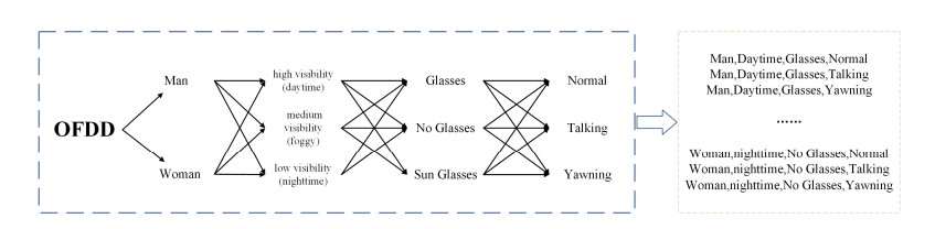
In recent years, UAV industry is developing rapidly and vigorously. However, so far, there is no relevant research on the fatigue detection method for UAV remote pilot, which is the core technology to ensure the flight safety of UAV. Aiming at this problem, a fatigue detection method for UAV remote pilot is proposed in this paper. Specifically, we first build a UAV operator fatigue detection database (OFDD). By analyzing the fatigue features in the database, we find that multiple facial features are highly correlated to the fatigue state, especially the head posture, and the temporal information is essential for distinguish between yawn and speaking in the study of UAV remote pilot fatigue detection. Based on these findings, a fatigue detection method for UAV remote pilots was proposed by efficiently locating the related facial regions, a multiple features extraction module to extract the eye, mouth and head posture features, and an efficient temporal fatigue decision module based on SVM. The experimental results show that this method not only performs well on the traditional driver dataset, but also achieves an accuracy rate of 97.05%; and it achieves the highest detection accuracy rate of 97.32% on the UAV remote pilots fatigue detection dataset OFDD.

Keywords:

Citation: Lei Pan, Chongyao Yan, Yuan Zheng, Qiang Fu, Yangjie Zhang, Zhiwei Lu, Zhiqing Zhao, Jun Tian. Fatigue detection method for UAV remote pilot based on multi feature fusion[J]. Electronic Research Archive, 2023, 31(1): 442-466. doi: 10.3934/era.2023022

Related Papers:

[1]	Haiming Liu, Jiajing Miao . Gauss-Bonnet theorem in Lorentzian Sasakian space forms. AIMS Mathematics, 2021, 6(8): 8772-8791. doi: 10.3934/math.2021509
[2]	Haiming Liu, Xiawei Chen, Jianyun Guan, Peifu Zu . Lorentzian approximations for a Lorentzian $\alpha$ -Sasakian manifold and Gauss-Bonnet theorems. AIMS Mathematics, 2023, 8(1): 501-528. doi: 10.3934/math.2023024
[3]	Lizhen Huang, Qunying Wu . Precise asymptotics for complete integral convergence in the law of the logarithm under the sub-linear expectations. AIMS Mathematics, 2023, 8(4): 8964-8984. doi: 10.3934/math.2023449
[4]	Xhevat Z. Krasniqi . Approximation of functions in a certain Banach space by some generalized singular integrals. AIMS Mathematics, 2024, 9(2): 3386-3398. doi: 10.3934/math.2024166
[5]	Shuyan Li, Qunying Wu . Complete integration convergence for arrays of rowwise extended negatively dependent random variables under the sub-linear expectations. AIMS Mathematics, 2021, 6(11): 12166-12181. doi: 10.3934/math.2021706
[6]	Najmeddine Attia, Rim Amami . On linear transformation of generalized affine fractal interpolation function. AIMS Mathematics, 2024, 9(7): 16848-16862. doi: 10.3934/math.2024817
[7]	Franka Baaske, Romaric Kana Nguedia, Hans-Jürgen Schmeißer . Smoothing properties of the fractional Gauss-Weierstrass semi-group in Morrey smoothness spaces. AIMS Mathematics, 2024, 9(11): 31962-31984. doi: 10.3934/math.20241536
[8]	Qiujin He, Chunxia Bu, Rongling Yang . A Generalization of Lieb concavity theorem. AIMS Mathematics, 2024, 9(5): 12305-12314. doi: 10.3934/math.2024601
[9]	Fethi Bouzeffour . Inversion formulas for space-fractional Bessel heat diffusion through Tikhonov regularization. AIMS Mathematics, 2024, 9(8): 20826-20842. doi: 10.3934/math.20241013
[10]	Iqra Shamas, Saif Ur Rehman, Thabet Abdeljawad, Mariyam Sattar, Sami Ullah Khan, Nabil Mlaiki . Generalized contraction theorems approach to fuzzy differential equations in fuzzy metric spaces. AIMS Mathematics, 2022, 7(6): 11243-11275. doi: 10.3934/math.2022628

Abstract

1. Introduction

In ^[4], Diniz and Veloso gave the definition of Gaussian curvature for non-horizontal surfaces in sub-Riemannian Heisenberg space $\mathbb{H}^1$ and the proof of the Gauss-Bonnet theorem. In ^[1], intrinsic Gaussian curvature for a Euclidean $C^2$ -smooth surface in the Heisenberg group $\mathbb{H}^1$ away from characteristic points and intrinsic signed geodesic curvature for Euclidean $C^2$ -smooth curves on surfaces are defined by using a Riemannian approximation scheme. These results were then used to prove a Heisenberg version of the Gauss-Bonnet theorem. In ^[5], Veloso verified that Gaussian curvature of surfaces and normal curvature of curves in surfaces introduced by ^[4] and by ^[1] to prove Gauss-Bonnet theorems in Heisenberg space $\mathbb{H}^1$ were unequal and he applied the same formalism of ^[4] to get the curvatures of ^[1]. With the obtained formulas, the Gauss-Bonnet theorem can be proved as a straightforward application of Stokes theorem in ^[5].

In ^[1] and ^[2], Balogh-Tyson-Vecchi used that the Riemannian approximation scheme may depend upon the choice of the complement to the horizontal distribution in general. In the context of $\mathbb{H}^1$ the choice which they have adopted is rather natural. The existence of the limit defining the intrinsic curvature of a surface depends crucially on the cancellation of certain divergent quantities in the limit. Such cancellation stems from the specific choice of the adapted frame bundle on the surface, and on symmetries of the underlying left-invariant group structure on the Heisenberg group. In ^[1], they proposed an interesting question to understand to what extent similar phenomena hold in other sub-Riemannian geometric structures. In ^[6], Wang and Wei gave sub-Riemannian limits of Gaussian curvature for a Euclidean $C^2$ -smooth surface in the affine group and the group of rigid motions of the Minkowski plane away from characteristic points and signed geodesic curvature for Euclidean $C^2$ -smooth curves on surfaces. And they got Gauss-Bonnet theorems in the affine group and the group of rigid motions of the Minkowski plane. In ^[7], Wang and Wei gave sub-Riemannian limits of Gaussian curvature for a Euclidean $C^2$ -smooth surface in the BCV spaces and the twisted Heisenberg group away from characteristic points and signed geodesic curvature for Euclidean $C^2$ -smooth curves on surfaces. And they got Gauss-Bonnet theorems in the BCV spaces and the twisted Heisenberg group.

In this paper, we solve this problem for the generalized affine group and the generalized BCV spaces. In the case of the generalized affine group, the cancellation of certain divergent quantities in the limit happens and the limit of the Riemannian Gaussian curvature exists. In the case of the generalized BCV spaces, the result is the same as the generalized affine group. We also get Gauss-Bonnet theorems in the generalized affine group and the generalized BCV spaces.

In Section 2, we compute the sub-Riemannian limit of curvature of curves in the generalized affine group. In Section 3, we compute sub-Riemannian limits of geodesic curvature of curves on surfaces and the Riemannian Gaussian curvature of surfaces in the generalized affine group. In Section 4, we prove the Gauss-Bonnet theorem in the generalized affine group. In Section 5, we compute the sub-Riemannian limit of curvature of curves in the generalized BCV spaces. In Section 6, we compute sub-Riemannian limits of geodesic curvature of curves on surfaces and the Riemannian Gaussian curvature of surfaces in the generalized BCV spaces and get a Gauss-Bonnet theorem in the generalized BCV spaces.

2. The sub-Riemannian limit of curvature of curves in the generalized affine group

When $TM = H\bigoplus H^\bot$ and $g^{TM} = g^H\bigoplus g^{H^\bot}$ , we may consider the rescaled metric $g_L = g^H\bigoplus Lg^{H^\bot}$ , then we may consider the sub-Riemannian limit of some geometric objects like the Gauss curvature and the mean curvature $\cdot\cdot\cdot$ , when L goes to the infinity. In this case, we call the $(M, g^{TM})$ as the manifold with the splitting tangent bundle. In this paper, our main objects $:$ the generalized affine group and the generalized BCV spaces are not sub-Riemannian manifolds (groups) in general. But they are manifolds with the splitting tangent bundle. So we can use the Riemannian approximation scheme to get the Gauss-Bonnet theorems in these spaces.

Firstly we give some notations on the generalized affine group. Let $\mathbb{G}$ be the generalized affine group and choose the underlying manifold $\mathbb{G} = \{(x_1, x_2, x_3)\in\mathbb{R}^3\mid f(x_1, x_2, x_3) > 0\}$ . On $\mathbb{G}$ , we let

$\begin{equation} X_1 = f\partial_{x_1}, \; \; X_2 = f\partial_{x_2}+\partial_{x_3}, \; \; X_3 = f\partial_{x_2}. \end{equation}$

(2.1)

where $f$ be a smooth function with respect to $x_1, x_2, x_3$ . Then

$\begin{equation} \partial_{x_1} = \frac{1}{f}X_1, \; \; \partial_{x_2} = \frac{1}{f}X_3, \; \; \partial_{x_3} = X_2-X_3, \end{equation}$

(2.2)

and ${\rm span}\{X_1, X_2, X_3\} = T\mathbb{G}.$ Let $H = {\rm span}\{X_1, X_2\}$ be the horizontal distribution on $\mathbb{G}$ . Let $\omega_1 = \frac{1}{f}dx_1, \; \; \omega_2 = dx_3, \; \; \omega = \frac{1}{f}dx_2-dx_3.$ Then $H = {\rm Ker}\omega$ . For the constant $L > 0$ , let $g_L = \omega_1\otimes \omega_1+\omega_2\otimes \omega_2+L\omega\otimes \omega, \; \; g = g_1$ be the Riemannian metric on $\mathbb{G}$ . Then $X_1, X_2, \widetilde{X_3}: = L^{-\frac{1}{2}}X_3$ are orthonormal basis on $T\mathbb{G}$ with respect to $g_L$ . We have

$\begin{equation} [X_1, X_2] = -(f_2+\frac{f_3}{f})X_1+f_1X_3, \; \; [X_1, X_3] = -f_2X_1+f_1X_3, \; \; [X_2, X_3] = \frac{f_3}{f}X_3. \end{equation}$

(2.3)

where $f_i = \frac{\partial{f}}{\partial x_i}$ , for $1\leq i\leq3.$

Let $\nabla^L$ be the Levi-Civita connection on $\mathbb{G}$ with respect to $g_L$ . Then we have the following lemma,

Lemma 2.1. Let $\mathbb{G}$ be the generalized affine group, then

$\begin{align} &\nabla^L_{X_1}X_1 = (f_2+\frac{f_3}{f})X_2+\frac{f_3}{L}, \; \; \; \nabla^L_{X_1}X_2 = -(f_2+\frac{f_3}{f})X_1+\frac{f_1}{2}X_3, \; \; \; \nabla^L_{X_2}X_1 = -\frac{f_1}{2}X_3, \\ &\nabla^L_{X_2}X_2 = 0, \nabla^L_{X_1}X_3 = -f_2X_1-\frac{f_1L}{2}X_2, \; \; \nabla^L_{X_3}X_1 = -\frac{f_1L}{2}X_2-f_1X_3, \\ &\nabla^L_{X_2}X_3 = \frac{f_1L}{2}X_1, \nabla^L_{X_3}X_2 = \frac{f_1L}{2}X_1-\frac{f_3}{f}X_3, \; \; \nabla^L_{X_3}X_3 = f_1LX_1+\frac{f_3L}{f}X_2. \end{align}$

(2.4)

Proof. By the Koszul formula, we have

$\begin{equation} 2\langle \nabla^L_{X_i}X_j, X_k\rangle_L = \langle[X_i, X_j], X_k\rangle_L-\langle[X_j, X_k], X_i\rangle_L+\langle[X_k, X_i], X_j\rangle_L, \end{equation}$

(2.5)

where $i, j, k = 1, 2, 3$ . So lemma 2.1 holds.

Definition 2.2. Let $\gamma:[a, b]\rightarrow (\mathbb{G}, g_L)$ be a Euclidean $C^1$ -smooth curve. We say that $\gamma$ is regular if $\dot{\gamma}\neq 0$ for every $t\in [a, b].$ Moreover we say that $\gamma(t)$ is a horizontal point of $\gamma$ if

$\omega(\dot{\gamma}(t)) = \frac{\dot{\gamma}_2(t)}{f}-\dot{\gamma}_3(t) = 0,$

where $\gamma(t) = (\gamma_1(t), \gamma_2(t), \gamma_3(t))$ and $\dot{\gamma}_i(t) = \frac{\partial\gamma_i(t)}{\partial t}$ .

Definition 2.3. Let $\gamma:[a, b]\rightarrow (\mathbb{G}, g_L)$ be a Euclidean $C^2$ -smooth regular curve in the Riemannian manifold $(\mathbb{G}, g_L)$ . The curvature $k^L_{\gamma}$ of $\gamma$ at $\gamma(t)$ is defined as

$\begin{equation} k^L_{\gamma}: = \sqrt{\frac{||\nabla^L_{\dot{\gamma}}{\dot{\gamma}}||_L^2}{||\dot{\gamma}||^4_L}-\frac{\langle \nabla^L_{\dot{\gamma}}{\dot{\gamma}}, \dot{\gamma}\rangle^2_L}{||\dot{\gamma}||^6_L}}. \end{equation}$

(2.6)

Lemma 2.4. Let $\gamma:[a, b]\rightarrow (\mathbb{G}, g_L)$ be a Euclidean $C^2$ -smooth regular curve in the Riemannian manifold $(\mathbb{G}, g_L)$ . Then,

$\begin{align} k^L_{\gamma}& = \Bigg\{\Bigg\{\left\{\left[\frac{\ddot{\gamma}_1-f_2\dot{\gamma}_1\dot{\gamma}_3}{f}-\frac{f'\dot{\gamma}_1+f_3\dot{\gamma}_1\dot{\gamma}_3}{f^2}\right]+\left[f_1L\dot{\gamma}_3-\frac{f_2\dot{\gamma}_1}{f}+f_1L\omega(\dot{\gamma}(t))\right]\omega(\dot{\gamma}(t))\right\}^2\\ &+\left\{\left[\ddot{\gamma}_3+\frac{f_2\dot{\gamma}_1^2}{f^2}+\frac{f_3\dot{\gamma}_1^2}{f^3}\right]+\left[\frac{f_3L\omega(\dot{\gamma}(t))}{f}-\frac{f_1L\dot{\gamma}_1}{f}\right]\omega(\dot{\gamma}(t))\right\}^2\\ &+L\left\{\frac{f_2\dot{\gamma}_1^2}{f^2L}-\left[\frac{f_1\dot{\gamma}_1}{f}+\frac{f_3\dot{\gamma}_3}{f}\right]\omega(\dot{\gamma}(t))+\frac{d}{dt}\omega(\dot{\gamma}(t))\right\}^2\Bigg\} \cdot\left[\left(\frac{\dot{\gamma}_1}{f}\right)^2+\dot{\gamma}_3^2+L(\omega(\dot{\gamma}(t)))^2\right]^{-2}\\ &-\left\{\left[\frac{\dot{\gamma}_1\ddot{\gamma}_1}{f^2}-\frac{f'\dot{\gamma}_1^2}{f^3}+\dot{\gamma}_3\ddot{\gamma}_3\right]+\frac{Ld\omega(\dot{\gamma}(t))}{dt}\omega(\dot{\gamma}(t))\right\}^2 \cdot\left[\left(\frac{\dot{\gamma}_1}{f}\right)^2+\dot{\gamma}_3^2+L(\omega(\dot{\gamma}(t)))^2\right]^{-3}\Bigg\}^{\frac{1}{2}}\\ \end{align}$

(2.7)

In particular, if $\gamma(t)$ is a horizontal point of $\gamma$ ,

$\begin{align} k^L_{\gamma}& = \Bigg\{\Bigg\{\left[\frac{\ddot{\gamma}_1-f_2\dot{\gamma}_1\dot{\gamma}_3}{f}-\frac{f'\dot{\gamma}_1+f_3\dot{\gamma}_1\dot{\gamma}_3}{f^2}\right]^2+\left[\ddot{\gamma}_3+\frac{f_2\dot{\gamma}_1^2}{f^2}+\frac{f_3\dot{\gamma}_1^2}{f^3}\right]^2\\ &+L\left[\frac{f_2\dot{\gamma}_1^2}{f^2L}+\frac{d}{dt}\omega(\dot{\gamma}(t))\right]^2\Bigg\} \cdot\left[\left(\frac{\dot{\gamma}_1}{f}\right)^2+\dot{\gamma}_3^2\right]^{-2}\\ &-\left[\frac{\dot{\gamma}_1\ddot{\gamma}_1}{f^2}-\frac{f'\dot{\gamma}_1^2}{f^3}+\dot{\gamma}_3\ddot{\gamma}_3\right]^2 \cdot\left[\left(\frac{\dot{\gamma}_1}{f}\right)^2+\dot{\gamma}_3^2\right]^{-3}\Bigg\}^{\frac{1}{2}}\\ \end{align}$

(2.8)

where $f' = \dot{\gamma}(f) = \frac{d}{dt}f(\gamma(t)).$

Proof. By (2.2), we have

$\begin{equation} \dot{\gamma}(t) = \frac{\dot{\gamma}_1}{f}X_1+\dot{\gamma}_3X_2+\omega(\dot{\gamma}(t))X_3. \end{equation}$

(2.9)

By Lemma 2.1 and (2.9), we have

$\begin{align} &\nabla^L_{\dot{\gamma}}X_1 = \left[\frac{ff_2\dot{\gamma_1}(t)+f_3\dot{\gamma_1}(t)}{f^2}-\frac{f_1L\omega(\dot{\gamma}(t))}{2}\right]X_2+\left[\frac{f_2\dot{\gamma_1}(t)}{fL}-\frac{f_1\dot{\gamma_3}(t)}{2}-f_1\omega(\dot{\gamma}(t))\right]X_3, \\ &\nabla^L_{\dot{\gamma}}X_2 = \left[-\frac{ff_2\dot{\gamma_1}(t)+f_3\dot{\gamma_1}(t)}{f^2}+\frac{f_1L\omega(\dot{\gamma}(t))}{2}\right]X_1+\left[-\frac{f_3\omega(\dot{\gamma}(t))}{f}+\frac{f_1\dot{\gamma}(t)}{2f}\right]X_3, \\ &\nabla^L_{\dot{\gamma}}X_3 = \left[-\frac{f_2\dot{\gamma_1}(t)}{f}+\frac{Lf_1\dot{\gamma_3}(t)}{2}+f_1L\omega(\dot{\gamma}(t))\right]X_1+\left[-\frac{f_1L\dot{\gamma}(t)}{2f}+\frac{f_3L\omega(\dot{\gamma}(t))}{f}\right]X_2. \end{align}$

(2.10)

By (2.9) and (2.10), we have

$\begin{align} \nabla^L_{\dot{\gamma}}\dot{\gamma}& = \left\{\left[\frac{\ddot{\gamma}_1-f_2\dot{\gamma}_1\dot{\gamma}_3}{f}-\frac{f'\dot{\gamma}_1+f_3\dot{\gamma}_1\dot{\gamma}_3}{f^2}\right]+\left[f_1L\dot{\gamma}_3-\frac{f_2\dot{\gamma}_1}{f}+f_1L\omega(\dot{\gamma}(t))\right]\omega(\dot{\gamma}(t))\right\}X_1\\ &+\left\{\left[\ddot{\gamma}_3+\frac{f_2\dot{\gamma}_1^2}{f^2}+\frac{f_3\dot{\gamma}_1^2}{f^3}\right]+\left[\frac{f_3L\omega(\dot{\gamma}(t))}{f}-\frac{f_1L\dot{\gamma}_1}{f}\right]\omega(\dot{\gamma}(t))\right\}X_2\\ &+\left\{\frac{f_2\dot{\gamma}_1^2}{f^2L}-\left(\frac{f_1\dot{\gamma}_1}{f}+\frac{f_3\dot{\gamma}_3}{f}\right)\omega(\dot{\gamma}(t))+\frac{d\omega(\dot{\gamma}(t))}{dt}\right\}X_3 \end{align}$

(2.11)

By (2.6), (2.9) and (2.11), we get Lemma 2.4.

Definition 2.5. Let $\gamma:[a, b]\rightarrow (\mathbb{G}, g_L)$ be a Euclidean $C^2$ -smooth regular curve in the Riemannian manifold $(\mathbb{G}, g_L)$ . We define the intrinsic curvature $k_{\gamma}^{\infty}$ of $\gamma$ at $\gamma(t)$ to be

$k_{\gamma}^{\infty}: = {\rm lim}_{L\rightarrow +\infty}k_{\gamma}^L,$

if the limit exists.

We introduce the following notation: for continuous functions $f_1, f_2:(0, +\infty)\rightarrow \mathbb{R}$ ,

$\begin{equation} f_1(L)\sim f_2(L), \; \; as \; \; L\rightarrow +\infty\Leftrightarrow {\rm lim}_{L\rightarrow +\infty}\frac{f_1(L)}{f_2(L)} = 1. \end{equation}$

(2.12)

Lemma 2.6. Let $\gamma:[a, b]\rightarrow (\mathbb{G}, g_L)$ be a Euclidean $C^2$ -smooth regular curve in the Riemannian manifold $(\mathbb{G}, g_L)$ . Then

$\begin{equation} k_{\gamma}^{\infty} = \frac{\sqrt{\left[f_1\dot{\gamma}_1-\frac{f_3\dot{\gamma}_2}{f}+f_3\dot{\gamma}_3\right]^2+(f_1\dot{\gamma}_2)^2}}{|f||\omega(\dot{\gamma}(t))|}, \; \; if \; \; \omega(\dot{\gamma}(t))\neq 0, \end{equation}$

(2.13)

$\begin{align} k^{\infty}_{\gamma}& = \Bigg\{\Bigg\{\left[\frac{\ddot{\gamma}_1-f_2\dot{\gamma}_1\dot{\gamma}_3}{f}-\frac{f'\dot{\gamma}_1+f_3\dot{\gamma}_1\dot{\gamma}_3}{f^2}\right]^2+\left[\ddot{\gamma}_3+\frac{f_2\dot{\gamma}_1^2}{f^2}+\frac{f_3\dot{\gamma}_1^2}{f^3}\right]^2\\ &+\left(\frac{f_2\dot{\gamma}_1^2}{f^2}\right)^2\Bigg\} \cdot\left[\left(\frac{\dot{\gamma}_1}{f}\right)^2+\dot{\gamma}_3^2\right]^{-2}\\ &-\left[\frac{\dot{\gamma}_1\ddot{\gamma}_1}{f^2}-\frac{f'\dot{\gamma}_1^2}{f^3}+\dot{\gamma}_3\ddot{\gamma}_3\right]^2 \cdot\left[\left(\frac{\dot{\gamma}_1}{f}\right)^2+\dot{\gamma}_3^2\right]^{-3}\Bigg\}^{\frac{1}{2}}\\ &\; \; if \; \; \omega(\dot{\gamma}(t)) = 0 \; \; \; and\; \; \; \frac{d}{dt}(\omega(\dot{\gamma}(t))) = 0, \\ \end{align}$

(2.14)

$\begin{equation} {\rm lim}_{L\rightarrow +\infty}\frac{k_{\gamma}^{L}}{\sqrt{L}} = \frac{|\frac{d}{dt}(\omega(\dot{\gamma}(t)))|}{\left(\frac{\dot{\gamma}_1}{f}\right)^2+\dot{\gamma}_3^2}, \; \; if \; \; \omega(\dot{\gamma}(t)) = 0 \; \; and\; \; \frac{d}{dt}(\omega(\dot{\gamma}(t)))\neq 0. \end{equation}$

(2.15)

Proof. Using the notation introduced in (2.12), when $\omega(\dot{\gamma}(t))\neq 0$ , we have

$||\nabla^L_{\dot{\gamma}}{\dot{\gamma}}||_L^2\sim \left(\frac{\omega(\dot{\gamma}(t))}{f}\right)^2\left\{\left[f_1\dot{\gamma}_1-\frac{f_3\dot{\gamma}_2}{f}+f_3\dot{\gamma}_3\right]^2+(f_1\dot{\gamma}_2)^2\right\}L^2, \; \; as\; \; L\rightarrow +\infty,$

$||\dot{\gamma}||^2_L\sim L\omega(\dot{\gamma}(t))^2, \; \; as\; \; L\rightarrow +\infty,$

$\langle \nabla^L_{\dot{\gamma}}{\dot{\gamma}}, \dot{\gamma}\rangle^2_L\sim O(L^2)\; \; as\; \; L\rightarrow +\infty.$

Therefore

$\frac{||\nabla^L_{\dot{\gamma}}{\dot{\gamma}}||_L^2}{||\dot{\gamma}||^4_L}\rightarrow \frac{\left\{\left[f_1\dot{\gamma}_1-\frac{f_3\dot{\gamma}_2}{f}+f_3\dot{\gamma}_3)\right]^2+(f_1\dot{\gamma}_2)^2\right\}}{f^2\omega(\dot{\gamma}(t))^2}, \; \; as\; \; L\rightarrow +\infty,$

$\frac{\langle \nabla^L_{\dot{\gamma}}{\dot{\gamma}}, \dot{\gamma}\rangle^2_L}{||\dot{\gamma}||^6_L}\rightarrow 0, \; \; as\; \; L\rightarrow +\infty.$

So by (2.6), we have (2.13). (2.14) comes from (2.8) and

$\frac{d}{dt}(\omega(\dot{\gamma}(t))) = 0.$

When $\omega(\dot{\gamma}(t)) = 0$ and $\frac{d}{dt}(\omega(\dot{\gamma}(t)))\neq 0,$

we have

$||\nabla^L_{\dot{\gamma}}{\dot{\gamma}}||_L^2\sim L[\frac{d}{dt}(\omega(\dot{\gamma}(t)))]^2, \; \; as\; \; L\rightarrow +\infty,$

$||\dot{\gamma}||^2_L = \left(\frac{\dot{\gamma}_1}{f}\right)^2+\dot{\gamma}_3^2,$

$\langle \nabla^L_{\dot{\gamma}}{\dot{\gamma}}, \dot{\gamma}\rangle^2_L = O(1)\; \; as\; \; L\rightarrow +\infty.$

By (2.6), we get (2.15).

3. The sub-Riemannian limit of geodesic curvature of curves on surfaces in the generalized affine group

We will say that a surface $\Sigma\subset(\mathbb{G}, g_L)$ is regular if $\Sigma$ is a Euclidean $C^2$ -smooth compact and oriented surface. In particular we will assume that there exists a Euclidean $C^2$ -smooth function $u:\mathbb{G}\rightarrow \mathbb{R}$ such that

$\Sigma = \{(x_1, x_2, x_3)\in \mathbb{G}:u(x_1, x_2, x_3) = 0\}$

and $u_{x_1}\partial_{x_1}+u_{x_2}\partial_{x_2}+u_{x_3}\partial_{x_3}\neq 0.$ Let $\nabla_Hu = X_1(u)X_1+X_2(u)X_2.$ A point $x\in\Sigma$ is called characteristic if $\nabla_Hu(x) = 0$ . We define the characteristic set $C(\Sigma): = \{x\in\Sigma|\nabla_Hu(x) = 0\}.$ Our computations will be local and away from characteristic points of $\Sigma$ . Let us define first

$p: = X_1u, \; \; \; \; q: = X_2u , \; \; {\rm and}\; \; r: = \widetilde{X}_3u.$

We then define

$\begin{align} &l: = \sqrt{p^2+q^2}, \; \; \; \; l_L: = \sqrt{p^2+q^2+r^2}, \; \; \; \; \overline{p}: = \frac{p}{l}, \\ &\overline{q}: = \frac{q}{l}, \; \; \; \; \overline{p_L}: = \frac{p}{l_L}, \; \; \; \; \overline{q_L}: = \frac{q}{l_L}, \; \; \; \; \overline{r_L}: = \frac{r}{l_L}. \end{align}$

(3.1)

In particular, $\overline{p}^2+\overline{q}^2 = 1$ . These functions are well defined at every non-characteristic point. Let

$\begin{align} v_L = \overline{p_L}X_1+\overline{q_L}X_2+\overline{r_L}\widetilde{X_3}, \; \; \; \; e_1 = \overline{q}X_1-\overline{p}X_2, \; \; \; \; e_2 = \overline{r_L}\; \; \overline{p}X_1+\overline{r_L}\; \; \overline{q}X_2-\frac{l}{l_L}\widetilde{X_3}, \end{align}$

(3.2)

then $v_L$ is the Riemannian unit normal vector to $\Sigma$ and $e_1, e_2$ are the orthonormal basis of $\Sigma$ . On $T\Sigma$ we define a linear transformation $J_L:T\Sigma\rightarrow T\Sigma$ such that

$\begin{equation} J_L(e_1): = e_2;\; \; \; \; J_L(e_2): = -e_1. \end{equation}$

(3.3)

For every $U, V\in T\Sigma$ , we define $\nabla^{\Sigma, L}_UV = \pi \nabla^{L}_UV$ where $\pi:T\mathbb{G}\rightarrow T\Sigma$ is the projection. Then $\nabla^{\Sigma, L}$ is the Levi-Civita connection on $\Sigma$ with respect to the metric $g_L$ . By (2.11), (3.2) and

$\begin{equation} \nabla^{\Sigma, L}_{\dot{\gamma}}\dot{\gamma} = \langle \nabla^L_{\dot{\gamma}}\dot{\gamma}, e_1\rangle_Le_1+\langle \nabla^L_{\dot{\gamma}}\dot{\gamma}, e_2\rangle_Le_2, \end{equation}$

(3.4)

we have

$\begin{align} \nabla^{\Sigma, L}_{\dot{\gamma}}\dot{\gamma}& = \Bigg\{\overline{q}\left[\left(\frac{\ddot{\gamma}_1-f_2\dot{\gamma}_1\dot{\gamma}_3}{f}-\frac{f'\dot{\gamma}_1+f_3\dot{\gamma}_1\dot{\gamma}_3}{f^2}\right)+\left(f_1L\dot{\gamma}_3-\frac{f_2\dot{\gamma}_1}{f}+f_1L\omega(\dot{\gamma}(t))\right)\omega(\dot{\gamma}(t))\right]\\ &-\overline{p}\left[\left(\ddot{\gamma}_3+\frac{f_2\dot{\gamma}_1^2}{f^2}+\frac{f_3\dot{\gamma}_1^2}{f^3}\right)-\left(\frac{f_1L\dot{\gamma}_1-f_3L\omega(\dot{\gamma}(t))}{f}\right)\omega(\dot{\gamma}(t))\right]\Bigg\}e_1\\ &+\Bigg\{\overline{r_L}\; \; \overline{p}\left[\left(\frac{\ddot{\gamma}_1-f_2\dot{\gamma}_1\dot{\gamma}_3}{f}-\frac{f'\dot{\gamma}_1+f_3\dot{\gamma}_1\dot{\gamma}_3}{f^2}\right)+\left(f_1L\dot{\gamma}_3-\frac{f_2\dot{\gamma}_1}{f}+f_1L\omega(\dot{\gamma}(t))\right)\omega(\dot{\gamma}(t))\right]\\ &+\overline{r_L}\; \; \overline{q}\left[\left( \ddot{\gamma}_3+\frac{f_2\dot{\gamma}_1^2}{f^2}+\frac{f_3\dot{\gamma}_1^2}{f^3}\right)-\left(\frac{f_1L\dot{\gamma}_1}{f}-\frac{f_3L\omega(\dot{\gamma}(t))}{f}\right)\omega(\dot{\gamma}(t))\right]\\ &-\frac{l}{l_L}L^{\frac{1}{2}}\left[\frac{f_2\dot{\gamma}_1^2}{f^2L}-\left(\frac{f_1\dot{\gamma}_1}{f}+\frac{f_3\dot{\gamma}_3}{f}\right)\omega(\dot{\gamma}(t))+\frac{d}{dt}(\omega(\dot{\gamma}(t)))\right]\Bigg\}e_2. \end{align}$

(3.5)

Moreover if $\omega(\dot{\gamma}(t)) = 0$ , then

$\begin{align} \nabla^{\Sigma, L}_{\dot{\gamma}}\dot{\gamma}& = \Bigg\{\overline{q}\left[\frac{\ddot{\gamma}_1-f_2\dot{\gamma}_1\dot{\gamma}_3}{f}-\frac{f'\dot{\gamma}_1+f_3\dot{\gamma}_1\dot{\gamma}_3}{f^2}\right]-\overline{p}\left[\ddot{\gamma}_3+\frac{f_2\dot{\gamma}_1^2}{f^2}+\frac{f_3\dot{\gamma}_1^2}{f^3}\right]\Bigg\}e_1\\ &+\Bigg\{\overline{r_L}\; \; \overline{p}\left[\frac{\ddot{\gamma}_1-f_2\dot{\gamma}_1\dot{\gamma}_3}{f}-\frac{f'\dot{\gamma}_1+f_3\dot{\gamma}_1\dot{\gamma}_3}{f^2}\right]+\overline{r_L}\; \; \overline{q}\left[ \ddot{\gamma}_3+\frac{f_2\dot{\gamma}_1^2}{f^2}+\frac{f_3\dot{\gamma}_1^2}{f^3}\right]\\ &-\frac{l}{l_L}L^{\frac{1}{2}}\left[\frac{f_2\dot{\gamma}_1^2}{f^2L}-\frac{d}{dt}(\omega(\dot{\gamma}(t)))\right]\Bigg\}e_2. \end{align}$

(3.6)

Definition 3.1. Let $\Sigma\subset(\mathbb{G}, g_L)$ be a regular surface. Let $\gamma:[a, b]\rightarrow \Sigma$ be a Euclidean $C^2$ -smooth regular curve. The geodesic curvature $k^L_{\gamma, \Sigma}$ of $\gamma$ at $\gamma(t)$ is defined as

$\begin{equation} k^L_{\gamma, \Sigma}: = \sqrt{\frac{||\nabla^{\Sigma, L}_{\dot{\gamma}}{\dot{\gamma}}||_{\Sigma, L}^2}{||\dot{\gamma}||^4_{\Sigma, L}}-\frac{\langle \nabla^{\Sigma, L}_{\dot{\gamma}}{\dot{\gamma}}, \dot{\gamma}\rangle^2_{\Sigma, L}}{||\dot{\gamma}||^6_{\Sigma, L}}}. \end{equation}$

(3.7)

Definition 3.2. Let $\Sigma\subset(\mathbb{G}, g_L)$ be a regular surface. Let $\gamma:[a, b]\rightarrow \Sigma$ be a Euclidean $C^2$ -smooth regular curve. We define the intrinsic geodesic curvature $k_{\gamma, \Sigma}^{\infty}$ of $\gamma$ at $\gamma(t)$ to be

$k_{\gamma, \Sigma}^{\infty}: = {\rm lim}_{L\rightarrow +\infty}k_{\gamma, \Sigma}^L,$

if the limit exists.

Lemma 3.3. Let $\Sigma\subset(\mathbb{G}, g_L)$ be a regular surface. Let $\gamma:[a, b]\rightarrow \Sigma$ be a Euclidean $C^2$ -smooth regular curve. Then

$\begin{equation} k_{\gamma, \Sigma}^{\infty} = \frac{|\overline{p}\left(f_1\dot{\gamma}_1-\frac{f_3\dot{\gamma}_2}{f}+f_3\dot{\gamma}_3\right)+\overline{q}f_1\dot{\gamma}_2|}{|f||\omega(\dot{\gamma}(t))|}, \; \; if \; \; \omega(\dot{\gamma}(t))\neq 0, \end{equation}$

(3.8)

$k^{\infty}_{\gamma, \Sigma} = 0, \; \; if \; \; \omega(\dot{\gamma}(t)) = 0, \; \; \; and\; \; \; \frac{d}{dt}(\omega(\dot{\gamma}(t))) = 0,$

$\begin{equation} {\rm lim}_{L\rightarrow +\infty}\frac{k_{\gamma, \Sigma}^{L}}{\sqrt{L}} = \frac{|\frac{d}{dt}(\omega(\dot{\gamma}(t)))|}{\left(\overline{q}\frac{\dot{\gamma}_1}{f}-\overline{p}\dot{\gamma}_3\right)^2}, \; \; if \; \; \omega(\dot{\gamma}(t)) = 0 \; \; \; and\; \; \; \frac{d}{dt}(\omega(\dot{\gamma}(t)))\neq 0. \end{equation}$

(3.9)

Proof. we know $\dot{\gamma}(t) = \dot{\gamma_1}(t)\partial x_1+\dot{\gamma_2}(t)\partial x_2+\dot{\gamma_3}(t)\partial x_3$ , then by (2.2), $\dot{\gamma}(t) = \frac{\dot{\gamma_1}(t)}{\gamma_1(t)}X_1+\gamma_3(t)X_2+\omega(\dot{\gamma}(t))X_3.$

Let

$\dot{\gamma}(t) = \lambda_1e_1+\lambda_2e_2.$

Then

$\begin{eqnarray} \begin{cases} \frac{\dot{\gamma_1}(t)}{\gamma_1(t)} = \lambda_1\overline{q}+\lambda_2\overline{r_L}\overline{p}\\[2pt] \dot{\gamma_3}(t) = -\lambda_1\overline{p}+\lambda_2\overline{r_L}\overline{q}\\[2pt] \omega(\dot{\gamma}(t)) = -\lambda_2\frac{l}{l_L}L^{-\frac{1}{2}}\\[2pt] \end{cases} \end{eqnarray}$

(3.10)

We have

$\begin{eqnarray} \begin{cases} \lambda_1 = \overline{q}\frac{\dot{\gamma_1}(t)}{\gamma_1(t)}-\overline{p}\dot{\gamma_3}(t)\\[2pt] \lambda_2 = -\lambda_2\frac{l_L}{l}L^{\frac{1}{2}}\omega(\dot{\gamma}(t))\\[2pt] \end{cases} \end{eqnarray}$

(3.11)

Thus $\dot{\gamma}\in T\Sigma$ , we have

$\begin{equation} \dot{\gamma} = (\overline{q}\frac{\dot{\gamma}_1}{f}-\overline{p}\dot{\gamma}_3)e_1-\frac{l_L}{l}L^{\frac{1}{2}}\omega(\dot{\gamma}(t))e_2. \end{equation}$

(3.12)

By (3.6), we have

$||\nabla^{\Sigma, L}_{\dot{\gamma}}\dot{\gamma}||^2_{L, \Sigma} = \Bigg\{\overline{q}\left[\left(\frac{\ddot{\gamma}_1-f_2\dot{\gamma}_1\dot{\gamma}_3}{f}-\frac{f'\dot{\gamma}_1+f_3\dot{\gamma}_1\dot{\gamma}_3}{f^2}\right)+\left(f_1L\dot{\gamma}_3-\frac{f_2\dot{\gamma}_1}{f}+f_1L\omega(\dot{\gamma}(t))\right)\omega(\dot{\gamma}(t))\right]\\ -\overline{p}\left[\left(\ddot{\gamma}_3+\frac{f_2\dot{\gamma}_1^2}{f^2}+\frac{f_3\dot{\gamma}_1^2}{f^3}\right)-\left(\frac{f_1L\dot{\gamma}_1-f_3L\omega(\dot{\gamma}(t))}{f}\right)\omega(\dot{\gamma}(t))\right]\Bigg\}^2\\ +\Bigg\{\overline{r_L}\; \; \overline{p}\left[\left(\frac{\ddot{\gamma}_1-f_2\dot{\gamma}_1\dot{\gamma}_3}{f}-\frac{f'\dot{\gamma}_1+f_3\dot{\gamma}_1\dot{\gamma}_3}{f^2}\right)+\left(f_1L\dot{\gamma}_3-\frac{f_2\dot{\gamma}_1}{f}+f_1L\omega(\dot{\gamma}(t))\right)\omega(\dot{\gamma}(t))\right]\\ +\overline{r_L}\; \; \overline{q}\left[\left( \ddot{\gamma}_3+\frac{f_2\dot{\gamma}_1^2}{f^2}+\frac{f_3\dot{\gamma}_1^2}{f^3}\right)-\left(\frac{f_1L\dot{\gamma}_1}{f}-\frac{f_3L\omega(\dot{\gamma}(t))}{f}\right)\omega(\dot{\gamma}(t))\right]\\ -\frac{l}{l_L}L^{\frac{1}{2}}\left[\frac{f_2\dot{\gamma}_1^2}{f^2L}-\left(\frac{f_1\dot{\gamma}_1}{f}+\frac{f_3\dot{\gamma}_3}{f}\right)\omega(\dot{\gamma}(t))+\frac{d}{dt}(\omega(\dot{\gamma}(t)))\right]\Bigg\}^2\\ \sim L^2\frac{\left[\overline{p}\left(f_1\dot{\gamma}_1-\frac{f_3\dot{\gamma}_2}{f}+f_3\dot{\gamma}_3\right)+\overline{q}f_1\dot{\gamma}_2\right]^2\omega(\dot{\gamma}(t))^2}{f^2}, \; \; \; \; {\rm as} \; \; \; \; L\rightarrow +\infty.$

(3.13)

Similarly, we have that when $\omega(\dot{\gamma}(t))\neq 0$ ,

$\begin{equation} ||\dot{\gamma}||_{\Sigma, L} = \sqrt{(\overline{q}\frac{\dot{\gamma}_1}{f}-\overline{p}\dot{\gamma}_3)^2+(\frac{l_L}{l})^2L\omega(\dot{\gamma}(t))^2}\sim L^{\frac{1}{2}}|\omega(\dot{\gamma}(t))| , \; \; \; \; {\rm as} \; \; \; \; L\rightarrow +\infty. \end{equation}$

(3.14)

By (3.6) and (3.12), we have

$\begin{align} &\langle \nabla^{\Sigma, L}_{\dot{\gamma}}{\dot{\gamma}}, \dot{\gamma}\rangle_{\Sigma, L}\\ & = \left(\overline{q}\frac{\dot{\gamma}_1}{f} -\overline{p}\dot{\gamma}_3\right)\cdot \Bigg\{\overline{q}\left[\left(\frac{\ddot{\gamma}_1-f_2\dot{\gamma}_1\dot{\gamma}_3}{f}-\frac{f'\dot{\gamma}_1+f_3\dot{\gamma}_1\dot{\gamma}_3}{f^2}\right) \\+\left(f_1L\dot{\gamma}_3-\frac{f_2\dot{\gamma}_1}{f}+f_1L\omega(\dot{\gamma}(t))\right)\omega(\dot{\gamma}(t))\right]\\ &-\overline{p}\left[\left(\ddot{\gamma}_3+\frac{f_2\dot{\gamma}_1^2}{f^2}+\frac{f_3\dot{\gamma}_1^2}{f^3}\right)-\left(\frac{f_1L\dot{\gamma}_1-f_3L\omega(\dot{\gamma}(t))}{f}\right)\omega(\dot{\gamma}(t))\right]\Bigg\}\\ &-\frac{l_L}{l}L^{\frac{1}{2}}\omega(\dot{\gamma}(t)) \cdot\Bigg\{\overline{r_L}\; \; \overline{p}\left[\left(\frac{\ddot{\gamma}_1-f_2\dot{\gamma}_1\dot{\gamma}_3}{f}-\frac{f'\dot{\gamma}_1+f_3\dot{\gamma}_1\dot{\gamma}_3}{f^2}\right)\\+\left(f_1L\dot{\gamma}_3-\frac{f_2\dot{\gamma}_1}{f}+f_1L\omega(\dot{\gamma}(t))\right)\omega(\dot{\gamma}(t))\right]\\ &+\overline{r_L}\; \; \overline{q}\left[\left( \ddot{\gamma}_3+\frac{f_2\dot{\gamma}_1^2}{f^2}+\frac{f_3\dot{\gamma}_1^2}{f^3}\right)-\left(\frac{f_1L\dot{\gamma}_1}{f}-\frac{f_3L\omega(\dot{\gamma}(t))}{f}\right)\omega(\dot{\gamma}(t))\right]\\ &-\frac{l}{l_L}L^{\frac{1}{2}}\left[\frac{f_2\dot{\gamma}_1^2}{f^2L}-\left(\frac{f_1\dot{\gamma}_1}{f}+\frac{f_3\dot{\gamma}_3}{f}\right)\omega(\dot{\gamma}(t))+\frac{d}{dt}(\omega(\dot{\gamma}(t)))\right]\Bigg\}\\ &\sim M_0L, \end{align}$

(3.15)

where $M_0$ does not depend on $L$ . By (3.7), (3.13)–(3.15), we get (3.8). When $\omega(\dot{\gamma}(t)) = 0$ and $\frac{d}{dt}(\omega(\dot{\gamma}(t))) = 0,$

we have

$||\nabla^{\Sigma, L}_{\dot{\gamma}}\dot{\gamma}||^2_{L, \Sigma} = \Bigg[\overline{q}\left(\frac{\ddot{\gamma}_1-f_2\dot{\gamma}_1\dot{\gamma}_3}{f}-\frac{f'\dot{\gamma}_1+f_3\dot{\gamma}_1\dot{\gamma}_3}{f^2}\right)-\overline{p}\left(\ddot{\gamma}_3+\frac{f_2\dot{\gamma}_1^2}{f^2}+\frac{f_3\dot{\gamma}_1^2}{f^3}\right)\Bigg]^2\\ +\Bigg[\overline{r_L}\; \; \overline{p}\left(\frac{\ddot{\gamma}_1-f_2\dot{\gamma}_1\dot{\gamma}_3}{f}-\frac{f'\dot{\gamma}_1+f_3\dot{\gamma}_1\dot{\gamma}_3}{f^2}\right) +\overline{r_L}\; \; \overline{q}\left( \ddot{\gamma}_3+\frac{f_2\dot{\gamma}_1^2}{f^2}+\frac{f_3\dot{\gamma}_1^2}{f^3}\right)-\frac{l}{l_L}L^{\frac{1}{2}}\frac{f_2\dot{\gamma}_1^2}{f^2L}\Bigg]^2\\ \sim \Bigg[\overline{q}\left(\frac{\ddot{\gamma}_1-f_2\dot{\gamma}_1\dot{\gamma}_3}{f}-\frac{f'\dot{\gamma}_1+f_3\dot{\gamma}_1\dot{\gamma}_3}{f^2}\right)-\overline{p}\left(\ddot{\gamma}_3+\frac{f_2\dot{\gamma}_1^2}{f^2}+\frac{f_3\dot{\gamma}_1^2}{f^3}\right)\Bigg]^2$

(3.16)

and

$\begin{equation} ||\dot{\gamma}||_{\Sigma, L} = |\overline{q}\frac{\dot{\gamma}_1}{f}-\overline{p}\dot{\gamma}_3|, \end{equation}$

(3.17)

$\langle \nabla^{\Sigma, L}_{\dot{\gamma}}{\dot{\gamma}}, \dot{\gamma}\rangle_{\Sigma, L} = \\ (\overline{q}\frac{\dot{\gamma}_1}{f} -\overline{p}\dot{\gamma}_3) \cdot\Bigg[\overline{q}\left(\frac{\ddot{\gamma}_1-f_2\dot{\gamma}_1\dot{\gamma}_3}{f}-\frac{f'\dot{\gamma}_1+f_3\dot{\gamma}_1\dot{\gamma}_3}{f^2}\right)-\overline{p}\left(\ddot{\gamma}_3+\frac{f_2\dot{\gamma}_1^2}{f^2}+\frac{f_3\dot{\gamma}_1^2}{f^3}\right)\Bigg]$

(3.18)

By (3.16)–(3.18) and (3.7), we get $k^{\infty}_{\gamma, \Sigma} = 0$ . When $\omega(\dot{\gamma}(t)) = 0$ and $\frac{d}{dt}(\omega(\dot{\gamma}(t)))\neq 0,$

we have

$||\nabla^{\Sigma, L}_{\dot{\gamma}}\dot{\gamma}||^2_{L, \Sigma}\sim L [\frac{d}{dt}(\omega(\dot{\gamma}(t)))]^2,$

$\langle \nabla^{\Sigma, L}_{\dot{\gamma}}{\dot{\gamma}}, \dot{\gamma}\rangle_{\Sigma, L} = O(1),$

so we get (3.9).

Definition 3.4. Let $\Sigma\subset(\mathbb{G}, g_L)$ be a regular surface. Let $\gamma:[a, b]\rightarrow \Sigma$ be a Euclidean $C^2$ -smooth regular curve. The signed geodesic curvature $k^{L, s}_{\gamma, \Sigma}$ of $\gamma$ at $\gamma(t)$ is defined as

$\begin{equation} k^{L, s}_{\gamma, \Sigma}: = \frac{\langle \nabla^{\Sigma, L}_{\dot{\gamma}}{\dot{\gamma}}, J_L(\dot{\gamma})\rangle_{\Sigma, L}}{||\dot{\gamma}||^3_{\Sigma, L}}, \end{equation}$

(3.19)

where $J_L$ is defined by (3.3).

Definition 3.5. Let $\Sigma\subset(\mathbb{G}, g_L)$ be a regular surface. Let $\gamma:[a, b]\rightarrow \Sigma$ be a Euclidean $C^2$ -smooth regular curve. We define the intrinsic geodesic curvature $k_{\gamma, \Sigma}^{\infty}$ of $\gamma$ at the non-characteristic point $\gamma(t)$ to be

$k_{\gamma, \Sigma}^{\infty, s}: = {\rm lim}_{L\rightarrow +\infty}k_{\gamma, \Sigma}^{L, s},$

if the limit exists.

Lemma 3.6. Let $\Sigma\subset(\mathbb{G}, g_L)$ be a regular surface. Let $\gamma:[a, b]\rightarrow \Sigma$ be a Euclidean $C^2$ -smooth regular curve. Then

$\begin{equation} k_{\gamma, \Sigma}^{\infty, s} = \frac{\overline{p}\left(f_1\dot{\gamma}_1-\frac{f_3\dot{\gamma}_2}{f}+f_3\dot{\gamma}_3\right)+\overline{q}f_1\dot{\gamma}_2}{|f\omega(\dot{\gamma}(t))|}, \; \; if \; \; \omega(\dot{\gamma}(t))\neq 0, \end{equation}$

(3.20)

$k^{\infty, s}_{\gamma, \Sigma} = 0, \; \; if \; \; \omega(\dot{\gamma}(t)) = 0, \; \; \; and\; \; \; \frac{d}{dt}(\omega(\dot{\gamma}(t))) = 0,$

$\begin{equation} {\rm lim}_{L\rightarrow +\infty}\frac{k_{\gamma, \Sigma}^{L, s}}{\sqrt{L}} = \frac{(-\overline{q}\frac{\dot{\gamma}_1}{f}+\overline{p}\dot{\gamma}_3)\frac{d}{dt}(\omega(\dot{\gamma}(t)))}{|\overline{q}\frac{\dot{\gamma}_1}{f}-\overline{p}\dot{\gamma}_3|^3}, \; \; if \; \; \omega(\dot{\gamma}(t)) = 0 \; \; \; and\; \; \; \frac{d}{dt}(\omega(\dot{\gamma}(t)))\neq 0. \end{equation}$

(3.21)

Proof. By (3.3) and (3.12), we have

$\begin{equation} J_L(\dot{\gamma}) = \frac{l_L}{l}L^{\frac{1}{2}}\omega(\dot{\gamma}(t))e_1+(\overline{q}\frac{\dot{\gamma}_1}{f}-\overline{p}\dot{\gamma}_3)e_2. \end{equation}$

(3.22)

By (3.5) and (3.22), we have

$\langle \nabla^{\Sigma, L}_{\dot{\gamma}}\dot{\gamma}, J_L(\dot{\gamma})\rangle_{L, \Sigma}\\ = \frac{l_L}{l}L^{\frac{1}{2}}\omega(\dot{\gamma}(t)) \Bigg\{\overline{q}\left[\left(\frac{\ddot{\gamma}_1-f_2\dot{\gamma}_1\dot{\gamma}_3}{f}-\frac{f'\dot{\gamma}_1+f_3\dot{\gamma}_1\dot{\gamma}_3}{f^2}\right)+\left(f_1L\dot{\gamma}_3-\frac{f_2\dot{\gamma}_1}{f}+f_1L\omega(\dot{\gamma}(t))\right)\omega(\dot{\gamma}(t))\right]\\ -\overline{p}\left[\left(\ddot{\gamma}_3+\frac{f_2\dot{\gamma}_1^2}{f^2}+\frac{f_3\dot{\gamma}_1^2}{f^3}\right)-\left(\frac{f_1L\dot{\gamma}_1-f_3L\omega(\dot{\gamma}(t))}{f}\right)\omega(\dot{\gamma}(t))\right]\Bigg\}\\ +(\overline{q}\frac{\dot{\gamma}_1}{f}-\overline{p}\dot{\gamma}_3)\cdot \Bigg\{\overline{r_L}\; \; \overline{p}\left[\left(\frac{\ddot{\gamma}_1-f_2\dot{\gamma}_1\dot{\gamma}_3}{f}-\frac{f'\dot{\gamma}_1+f_3\dot{\gamma}_1\dot{\gamma}_3}{f^2}\right)\\+\left(f_1L\dot{\gamma}_3-\frac{f_2\dot{\gamma}_1}{f}+f_1L\omega(\dot{\gamma}(t))\right)\omega(\dot{\gamma}(t))\right]\\ +\overline{r_L}\; \; \overline{q}\left[\left( \ddot{\gamma}_3+\frac{f_2\dot{\gamma}_1^2}{f^2}+\frac{f_3\dot{\gamma}_1^2}{f^3}\right)-\left(\frac{f_1L\dot{\gamma}_1}{f}-\frac{f_3L\omega(\dot{\gamma}(t))}{f}\right)\omega(\dot{\gamma}(t))\right]\\ -\frac{l}{l_L}L^{\frac{1}{2}}\left[\frac{f_2\dot{\gamma}_1^2}{f^2L}-\left(\frac{f_1\dot{\gamma}_1}{f}+\frac{f_3\dot{\gamma}_3}{f}\right)\omega(\dot{\gamma}(t))+\frac{d}{dt}(\omega(\dot{\gamma}(t)))\right]\Bigg\}, \\ \sim L^{\frac{3}{2}}\omega(\dot{\gamma}(t))^2\frac{\overline{p}\left(f_1\dot{\gamma}_1-\frac{f_3\dot{\gamma}_2}{f}+f_3\dot{\gamma}_3\right)+\overline{q}f_1\dot{\gamma}_2}{f}\; \; {\rm as}\; \; L\rightarrow +\infty.$

(3.23)

So we get (3.20). When $\omega(\dot{\gamma}(t)) = 0$ and $\frac{d}{dt}(\omega(\dot{\gamma}(t))) = 0,$ we get

$\begin{align} &\langle \nabla^{\Sigma, L}_{\dot{\gamma}}\dot{\gamma}, J_L(\dot{\gamma})\rangle_{L, \Sigma}\\ & = (\overline{q}\frac{\dot{\gamma}_1}{f}-\overline{p}\dot{\gamma}_3)\cdot \left[\overline{r_L}\; \; \overline{p}\left(\frac{\ddot{\gamma}_1-f_2\dot{\gamma}_1\dot{\gamma}_3}{f}-\frac{f'\dot{\gamma}_1+f_3\dot{\gamma}_1\dot{\gamma}_3}{f^2}\right)\\+\overline{r_L}\; \; \overline{q}\left(\ddot{\gamma}_3+\frac{f_2\dot{\gamma}_1^2}{f^2}+\frac{f_3\dot{\gamma}_1^2}{f^3}\right)-\frac{l}{l_L}L^{-\frac{1}{2}}\frac{f_2\dot{\gamma}_1^2}{f^2}\right]\\ &\sim M_0L^{-\frac{1}{2}}\; \; {\rm as}\; \; L\rightarrow +\infty. \end{align}$

(3.24)

So $k^{\infty, s}_{\gamma, \Sigma} = 0.$ When $\omega(\dot{\gamma}(t)) = 0$ and $\frac{d}{dt}(\omega(\dot{\gamma}(t)))\neq0,$

we have

$\begin{align} \langle \nabla^{\Sigma, L}_{\dot{\gamma}}\dot{\gamma}, J_L(\dot{\gamma})\rangle_{L, \Sigma}\sim L^{\frac{1}{2}}(-\overline{q}\frac{\dot{\gamma}_1}{f}+\overline{p}\dot{\gamma}_3)\frac{d}{dt}(\omega(\dot{\gamma}(t)))\; \; {\rm as}\; \; L\rightarrow +\infty. \end{align}$

(3.25)

So we get (3.21).

In the following, we compute the sub-Riemannian limit of the Riemannian Gaussian curvature of surfaces in the generalized affine group. We define the second fundamental form $II^L$ of the embedding of $\Sigma$ into $(\mathbb{G}, g_L)$ :

$\begin{equation} II^L = \left( \begin{array}{cc} \langle \nabla^{L}_{e_1}v_L, e_1\rangle_{L}, & \langle \nabla^{L}_{e_1}v_L, e_2\rangle_{L} \\ \langle \nabla^{L}_{e_2}v_L, e_1\rangle_{L}, & \langle \nabla^{L}_{e_2}v_L, e_2\rangle_{L} \\ \end{array} \right). \end{equation}$

(3.26)

Similarly to Theorem 4.3 in ^[3], we have

Theorem 3.7. The second fundamental form $II^L$ of the embedding of $\Sigma$ into $(\mathbb{G}, g_L)$ is given by

$\begin{equation} II^L = \left( \begin{array}{cc} h_{11}, & h_{12} \\ h_{21} , & h_{22} \\ \end{array} \right). \end{equation}$

(3.27)

where

$h_{11} = \frac{l}{l_L}[X_1(\overline{p})+X_2(\overline{q})]-\overline{q_L}\left(f_2+\frac{f_3}{f}\right)-\overline{q}^2f_2\overline{r_L}L^{-\frac{1}{2}},$

$h_{12} = h_{21} = -\frac{l_L}{l}\langle e_1, \nabla_H(\overline{r_L})\rangle_L-\frac{f_1\sqrt{L}}{2}-\overline{p}\overline{q}f_2L^{-\frac{1}{2}},$

$h_{22} = -\frac{l^2}{l_L^2}\langle e_2, \nabla_H(\frac{r}{l})\rangle_L+\widetilde{X_3}(\overline{r_L})-f_1\overline{p_L}-\overline{q_L}\frac{f_3}{f}-\overline{r_L}\overline{P}^2f_2L^{-\frac{1}{2}}.$

Proof. By $e_i\langle V_L, e_j\rangle_L-\langle\nabla^L_{e_i}V_L, e_j\rangle_L-\langle\nabla^L_{e_i}e_j, V_L\rangle_L = 0$ and $e_i\langle V_L, e_j\rangle_L = 0$ , we have $\langle\nabla^L_{e_i}V_L, e_j\rangle_L = -\langle\nabla^L_{e_i}e_j, V_L\rangle_L,$ $i, j = 1, 2$ .

By lemma 2.1 and (3.2),

$\begin{align} \nabla^L_{e_1}e_1& = \nabla^L_{(\overline{q}X_1-\overline{p}X_2)}(\overline{q}X_1-\overline{p}X_2)\\ & = [\overline{q}X_1(\overline{q})-\overline{p}X_2(\overline{p})+\overline{p}\overline{q}(f_2+\frac{f_3}{f})]X_1\\ &-[\overline{q}X_1(\overline{p})-\overline{p}X_2(\overline{p})-\overline{q}^2(f_2+\frac{f_3}{f})]X_2+\overline{q}^2f_3L^{-\frac{1}{2}}\widetilde{X_3}.\\ \end{align}$

(3.28)

Then

$\begin{align} h_{11}& = -\langle\nabla^L_{e_1}e_1, V_L\rangle_L\\ & = -\overline{p_L}[\overline{q}X_1(\overline{q})-\overline{p}X_2(\overline{p})]+\overline{q_L}[\overline{q}X_1(\overline{p})-\overline{p}X_2(\overline{p})]\\ &-\overline{q_L}\left(F_2+\frac{F_3\overline{f}}{F}\right)-\overline{p_L}\left(F_1+\frac{F_3f}{F}\right)+\overline{r_L}L^{-\frac{1}{2}}\frac{F_3}{F}\\ & = \frac{l}{l_L}[X_1(\overline{p})+X_2(\overline{q})]-\overline{q_L}\left(F_2+\frac{F_3\overline{f}}{F}\right)-\overline{p_L}\left(F_1+\frac{F_3f}{F}\right)+\overline{r_L}L^{-\frac{1}{2}}\frac{F_3}{F}.\\ \end{align}$

(3.29)

Similarly,

$\begin{align} \nabla^L_{e_1}e_2& = \nabla^L_{(\overline{q}X_1-\overline{p}X_2)}(\overline{r_L}\overline{p}X_1+\overline{r_L}\overline{q}X_2-\frac{l}{l_L}\widetilde{X_3})\\ & = [\overline{q}X_1(\overline{r_L}\overline{p})-\overline{p}X_2(\overline{r_L}\overline{p})+\frac{f_1\overline{p_L}\sqrt{L}}{2}\\ &-\overline{r_L}\overline{q}^2(f_2+{f_3}{f})+\overline{q_L}f_2L^{-\frac{1}{2}}]X_1\\ &+[\overline{q}X_1(\overline{q})-\overline{p}X_2(\overline{q})+\frac{f_1\overline{q_L}\sqrt{L}}{2}\\ &+\overline{r_L}\overline{pq}(f_2+\frac{f_3}{f})]X_2\\ &+[\overline{p}X_2(\frac{l}{l_L})-\overline{q}X_1(\frac{l}{l_L})+\frac{f_1\overline{r_L}\sqrt{L}}{2}+\overline{r_L}\overline{pq}f_3L^{-\frac{1}{2}}]\widetilde{X_3}.\\ \end{align}$

(3.30)

Then

$\begin{align} h_{12}& = -\langle\nabla^L_{e_1}e_2, V_L\rangle_L\\ & = -\frac{l}{l_L}[\overline{q}X_1(\overline{r_L})-\overline{p}X_2(\overline{r_L})]\\ &+\overline{r_L}[\overline{q}X_1(\frac{l}{l_L})-\overline{p}X_2(\frac{l}{l_L})]-\frac{1}{2}L^\frac{1}{2}(fF_2-F_1\overline{f}+\overline{f}'F-Ff')\\ & = -\frac{l_L}{l}\langle e_1, \nabla_H(\overline{r_L})\rangle_L-\frac{1}{2}L^\frac{1}{2}(fF_2-F_1\overline{f}+\overline{f}'F-Ff').\\ \end{align}$

(3.31)

Since

$\begin{align} \langle\nabla^L_{e_2}V_L, e_1\rangle_L& = -\langle\nabla^L_{e_2}e_1, V_L\rangle_L = -\langle\nabla^L_{e_1}e_2+[e_2, e_1], V_L\rangle_L\\ & = -\langle\nabla^L_{e_1}e_2, V_L\rangle = \langle\nabla^L_{e_1}V_L, e_2\rangle_L.\\ \end{align}$

(3.32)

Then,

$\begin{align} h_{21} = h_{12} = -\frac{l_L}{l}\langle e_1, \nabla_H(\overline{r_L})\rangle_L-\frac{1}{2}L^\frac{1}{2}(fF_2-F_1\overline{f}+\overline{f}'F-Ff').\\ \end{align}$

(3.33)

Since

$\begin{align} \nabla^L_{e_2}e_2& = \nabla^L_{(\overline{r_L}\overline{p}X_1+\overline{r_L}\overline{q}X_2-\frac{l}{l_L}\widetilde{X_3})}(\overline{r_L}\overline{p}X_1+\overline{r_L}\overline{q}X_2-\frac{l}{l_L}\widetilde{X_3})\\ & = [\overline{q}X_1(\overline{r_L}\overline{p})-\overline{p}X_2(\overline{r_L}\overline{p})+f_1\overline{q_L}\sqrt{L}-\overline{r_L}^2\overline{pq}(f_2+\frac{f_3}{f})\\ &+\overline{r_L}\overline{p_L}f_2L^{-\frac{1}{2}}+(\frac{l}{l_L})^2f_1]X_1\\ &+[\overline{q}X_1(\overline{q})-\overline{p}X_2(\overline{q})+f_1\overline{p_L}\sqrt{L}+\overline{r_L}^2\overline{pq}(f_2+{f_3}{f})+(\frac{l}{l_L})^2\frac{f_3}{f}X_2\\ &+[\overline{p}X_2(\frac{l}{l_L})-\overline{q}X_1(\frac{l}{l_L})+\overline{r_L}^2\overline{pq}\frac{f_3}{f}L^{-\frac{1}{2}}+\overline{r_L}\overline{p_L}f_1+\overline{r_L}\overline{q_L}\frac{f_3}{f}]\widetilde{X_3}.\\ \end{align}$

(3.34)

Then,

$\begin{align} h_{22}& = -\langle\nabla^L_{e_2}e_2, V_L\rangle_L\\ & = -\overline{p}\frac{r}{l}X_1(\overline{r_L})-\overline{q}\frac{r}{l}X_2(\overline{r_L})+\widetilde{X_3}(\overline{r_L})-\overline{p_L}\frac{fF_3}{F}-\overline{q_L}\frac{\overline{f}F_3}{F}-\overline{r_L}\frac{F_3}{F}L^{-\frac{1}{2}}\\ & = -\frac{l^2}{l_L^2}\langle e_2, \nabla_H(\frac{r}{l})\rangle_L+\widetilde{X_3}(\overline{r_L})-\overline{p_L}\frac{fF_3}{F}-\overline{q_L}\frac{\overline{f}F_3}{F}-\overline{r_L}\frac{F_3}{F}L^{-\frac{1}{2}} .\\ \end{align}$

(3.35)

The Riemannian mean curvature $\mathcal{H}_L$ of $\Sigma$ is defined by

$\mathcal{H}_L: = {\rm tr}(II^L).$

Let

$\begin{equation} \mathcal{K}^{\Sigma, L}(e_1, e_2) = -\langle R^{\Sigma, L}(e_1, e_2)e_1, e_2\rangle_{\Sigma, L}, \; \; \; \; \mathcal{K}^{L}(e_1, e_2) = -\langle R^{L}(e_1, e_2)e_1, e_2\rangle_L. \end{equation}$

(3.36)

By the Gauss equation, we have

$\begin{equation} \mathcal{K}^{\Sigma, L}(e_1, e_2) = \mathcal{K}^{L}(e_1, e_2)+{\rm det}(II^L). \end{equation}$

(3.37)

Proposition 3.8. Away from characteristic points, the horizontal mean curvature $\mathcal{H}_{\infty}$ of $\Sigma\subset\mathbb{G}$ is given by

$\begin{equation} \mathcal{H}_{\infty} = {\rm lim}_{L\rightarrow +\infty}\mathbb{}\mathcal{H}_L = X_1(\overline{p})+X_2(\overline{q})-f_1\overline{p}-\overline{q}f_2-2\overline{q}\frac{f_3}{f}. \end{equation}$

(3.38)

Proof. By

$\frac{l^2}{l_L^2}\langle e_2, \nabla_H(\frac{r}{l})\rangle_L = \frac{\overline{p}r}{l}X_1(\overline{r_L})+\frac{\overline{q}r}{l}X_2(\overline{r_L}) = O(L^{-1})$

$\frac{l}{l_L}[X_1(\overline{p})+X_2(\overline{q})]\rightarrow X_1(\overline{p})+X_2(\overline{q}), \; \; \; \; \widetilde{X_3}(\overline{r_L})\rightarrow 0,$

$\overline{q}^2f_2\overline{r_L}L^{-\frac{1}{2}}\rightarrow O(L^{-1}), \; \; \; \; \overline{q_L}\rightarrow \overline{q},$

$\overline{r_L}\overline{P}^2f_2L^{-\frac{1}{2}}\rightarrow O(L^{-1}), \; \; \; \; \overline{p_L}\rightarrow \overline{p},$

we get (3.38).

Define the curvature of a connection $\nabla$ by

$\begin{equation} R(X, Y)Z = \nabla_X\nabla_YZ-\nabla_Y\nabla_XZ-\nabla_{[X, Y]}Z. \end{equation}$

(3.39)

Then by Lemma 2.1 and (3.39), we have the following lemma,

Lemma 3.9. Let $\mathbb{G}$ be the affine group, then

$\ R^L(X_1, X_2)X_1 = \left[\frac{3Lf_1^2}{4}+\left(f_2+\frac{f_3}{f}\right)^2\right]X_2+\left[X_1\left(-\frac{f_1}{2}\right)-X_2\left(\frac{f_2}{L}\right)+f_1^2+\frac{f_2^2}{L}+\frac{f_2f_3}{Lf}\right]X_3, \\ R^L(X_1, X_2)X_2 = \left[-\frac{3Lf_1^2}{4}+X_2\left(f_2+\frac{f_3}{f}\right)-\left(f_2+\frac{f_3}{f}\right)^2\right]X_1+\frac{f_1f_3}{f}X_3, \\ R^L(X_1, X_2)X_3 = \left[X_1\left(\frac{f_1L}{2}\right)+X_2(f_2)-f_1^2L-f_2\left(f_2+\frac{f_3}{f}\right)\right]X_1+\left[X_2\left(\frac{f_1L}{f}\right)-\frac{f_1f_3L}{f}\right]X_2, \\ R^L(X_1, X_3)X_1 = -\left[X_1\left(\frac{f_1L}{2}\right)+X_3\left(f_2+\frac{f_3}{f}\right)+\frac{f_2f_3}{f}-f_1^2L-f_2\left(f_2+\frac{f_3}{f}\right)\right]X_2\\ +\left[-\frac{f_1^2L}{4}+f_1^2+\frac{f_2^2}{L}-X_3\left(\frac{f_2}{L}\right)-X_1(f_1)+\frac{f_3}{f}\left(f_2+\frac{f_3}{f}\right)\right]X_3, \\ R^L(X_1, X_3)X_2 = \left[X_1\left(\frac{f_1L}{2}\right)-f_1^2L-f_2\left(f_2+\frac{f_3}{f}\right)+X_3\left(f_2+\frac{f_3}{f}\right)+\frac{f_2f_3}{f}\right]X_1\\ +\left[-X_1\left(\frac{f_3}{f}\right)+f_1f_2+\frac{f_1f_3}{f}-f_1\left(f_2+\frac{f_3}{f}\right)-X_3\left(\frac{f_1}{2}\right)\right]X_3, \\ R^L(X_1, X_3)X_3 = \left[X_1(f_1L)-\frac{f_3L}{f}\left(f_2+\frac{f_3}{f}\right)+X_3(f_2)+\frac{f_1^2L^2}{4}-f_1^2L-f_2^2\right]X_1\; \; \; \\ +\left[f_1L\left(f_2+\frac{f_3}{f}\right)+X_1\left(\frac{f_3L}{f}\right)-f_1f_2L-\frac{f_1f_3L}{f}+X_3\left(\frac{f_1L}{2}\right)\right]X_2, \\ R^L(X_2, X_3)X_1 = \left[-X_2\left(\frac{f_1L}{2}\right)+\frac{f_1f_3L}{f}\right]X_2+\left[X_3\left(\frac{f_1}{2}\right)-X_2(f_1)+\frac{f_1f_3}{f}\right]X_3, \\ R^L(X_2, X_3)X_2 = \left[X_2\left(\frac{f_1L}{2}\right)-\frac{f_1f_3L}{f}\right]X_1+\left[\frac{f_3^2}{f^2}-\frac{f_1^2L}{4}-X_2\left(\frac{f_3}{f}\right)\right]X_3, \\ R^L(X_2, X_3)X_3 = \left[X_2(f_1L)-X_3\left(\frac{f_1L}{2}\right)-\frac{f_1f_3L}{f}\right]X_1+\left[X_2\left(\frac{f_3L}{f}\right)-\frac{f_3^2L}{f^2}+\frac{f_1^2L^2}{4}\right]X_2.$

(3.40)

Proposition 3.10. Away from characteristic points, we have

$\begin{equation} \mathcal{K}^{\Sigma, L}(e_1, e_2)\rightarrow A_0+O(L^{-\frac{1}{2}}), \; \; {\rm as}\; \; L\rightarrow +\infty, \end{equation}$

(3.41)

where

$\begin{align} A_0&: = -f_1\langle e_1, \nabla_H(\frac{X_3u}{|\nabla_Hu|})\rangle-f_1f_2\overline{p}\overline{q}-\overline{q}^2f_1^2-\frac{3}{4}\frac{(X_3u)^2}{l^2}f_1^2+\overline{p}^2X_2(\frac{f_3}{f})\\ &-\overline{p}\left[X_1(\overline{p})+X_2(\overline{q})-\overline{q}\left(f_2+\frac{f_3}{f}\right)\right]\left(f_1\overline{p}+\overline{q}\frac{f_3}{f}\right)\\ &+2\overline{q}\frac{X_3u}{l}f_1^2+2\overline{q}\frac{X_3u}X_1(-\frac{f_1}{2})-2\overline{p}\frac{X_3u}{l}\frac{f_1f_3}{f}+\overline{q}^2X_1(f_1)\\ &-\overline{q}^2\left(f_2+\frac{f_3}{f}\right)-2\overline{q}\overline{p}X_1(\frac{f_3}{f})-2\overline{q}\overline{p}X_3(\frac{f_1}{2})-\overline{p}^2\frac{f_3^2}{f^2}. \end{align}$

(3.42)

Proof. By (3.2), we have

$\begin{align} &\; \; \; \; \langle R^{L}(e_1, e_2)e_1, e_2\rangle_L\\ & = \overline{r_L}^2\langle R^{L}(X_1, X_2)X_1, X_2\rangle_L-2\frac{l}{l_L}\overline{q}L^{-\frac{1}{2}}\overline{r_L}\langle R^{L}(X_1, X_2)X_1, X_3\rangle_L\\ &+2\frac{l}{l_L}\overline{p}L^{-\frac{1}{2}}\overline{r_L}\langle R^{L}(X_1, X_2)X_2, X_3\rangle_L+(\frac{l}{l_L}\overline{q})^2L^{-1}\langle R^{L}(X_1, X_3)X_1, X_3\rangle_L\\ &-2(\frac{l}{l_L})^2\overline{p}\overline{q}L^{-1}\langle R^{L}(X_1, X_3)X_2, X_3\rangle_L+(\overline{p}\frac{l}{l_L})^2L^{-1}\langle R^{L}(X_2, X_3)X_2, X_3\rangle_L.\\ \end{align}$

(3.43)

By Lemma 3.9, we have

$\begin{align} \mathcal{K}^{L}(e_1, e_2)& = \frac{1}{4}\frac{l^2}{l_L^2}f_1^2L-\frac{3}{4}Lf_1^2\overline{r_L}^2+2\frac{l}{l_L}\overline{q}L^{\frac{1}{2}}\overline{r_L}f_1^2-\overline{q}^2\frac{l^2}{l_L^2}f_1^2\\ &-\overline{r_L}^2\left(f_2+\frac{f_3}{f}\right)^2+2\frac{l}{l_L}\overline{q}L^\frac{1}{2}\overline{r_L}X_1\left(-\frac{f_1}{2}\right)-2\frac{l}{l_L}\overline{q}L^\frac{1}{2}\overline{r_L}X_2\left(-\frac{f_2}{L}\right)\\ &+2\frac{l}{l_L}\overline{q}L^{-\frac{1}{2}}\overline{r_L}f_2^2+2\frac{l}{l_L}\overline{q}L^{-\frac{1}{2}}\overline{r_L}\frac{f_2f_3}{f}-2\overline{p}L^\frac{1}{2}\overline{r_L}\frac{f_1f_3}{f}\\ &-\overline{q}^2\frac{l^2}{l_L^2}\frac{f_2^2}{L}+\overline{q}^2\frac{l^2}{l_L^2}X_3\left(\frac{f_2}{L}\right)+\overline{q}^2\frac{l^2}{l_L^2}X_1\left(f_1\right)-\overline{q}^2\frac{l^2}{l_L^2}\left(f_2+\frac{f_3}{f}\right)\\ &-2\overline{qp}\frac{l^2}{l_L^2}X_1\left(\frac{f_3}{f}\right)+2\overline{qp}\frac{l^2}{l_L^2}f_1f_2+2\overline{qp}\frac{l^2}{l_L^2}\frac{f_1f_3}{f}-2\overline{qp}\frac{l^2}{l_L^2}f_1\left(f_2+\frac{f_3}{f}\right)\\ &-2\overline{qp}\frac{l^2}{l_L^2}X_3\left(\frac{f_1}{2}\right)-\overline{p}^2\frac{l^2}{l_L^2}\frac{f_3^2}{f^2}+\overline{p}^2\frac{l^2}{l_L^2}X_2\left(\frac{f_3}{f}\right). \end{align}$

(3.44)

By (3.35) and

$\nabla_H(\overline{r_L}) = L^{-\frac{1}{2}}\nabla_H(\frac{X_3u}{|\nabla_Hu|})+O(L^{-1})\; \; {\rm as}\; \; L\rightarrow +\infty$

we get

$\begin{align} {\rm det}(II^L)& = h_{11}h_{22}-h_{12}h_{21}\\ & = -\frac{f_1^2L}{4}-f_1\langle e_1, \nabla_H(\frac{X_3u}{|\nabla_Hu|})\rangle-f_1f_2\overline{p}\overline{q}\\ &-\overline{p}\left[X_1(\overline{p})+X_2(\overline{q})-\overline{q}\left(f_2+\frac{f_3}{f}\right)\right]\left(f_1\overline{p}+\overline{q}\frac{f_3}{f}\right) +O(L^{-\frac{1}{2}}). \end{align}$

(3.45)

By (3.38), (3.44), (3.45) we get (3.41).

4. A Gauss-Bonnet theorem in the generalized affine group

Let us first consider the case of a regular curve $\gamma:[a, b]\rightarrow (\mathbb{G}, g_L)$ . We define the Riemannian length measure

$ds_L = ||\dot{\gamma}||_Ldt.$

Lemma 4.1. Let $\gamma:[a, b]\rightarrow (\mathbb{G}, g_L)$ be a Euclidean $C^2$ -smooth and regular curve. Let

$\begin{equation} d{s}: = |\omega(\dot{\gamma}(t))|dt, \; \; \; \; d\overline{s}: = \frac{1}{2}\frac{1}{|\omega(\dot{\gamma}(t))|}\left(\frac{\dot{\gamma}_1^2}{f^2}+\dot{\gamma}_3^2\right)dt. \end{equation}$

(4.1)

Then

$\begin{equation} {\rm lim}_{L\rightarrow +\infty}\frac{1}{\sqrt{L}}\int_{\gamma}ds_L = \int_a^bds. \end{equation}$

(4.2)

When $\omega(\dot{\gamma}(t))\neq 0$ , we have

$\begin{equation} \frac{1}{\sqrt{L}}ds_L = ds+d\overline{s}L^{-1}+O(L^{-2}) \; \; {\rm as}\; \; L\rightarrow +\infty. \end{equation}$

(4.3)

When $\omega(\dot{\gamma}(t)) = 0$ , we have

$\begin{equation} \frac{1}{\sqrt{L}}ds_L = \frac{1}{\sqrt{L}}\sqrt{\frac{\dot{\gamma}_1^2}{f^2}+\dot{\gamma}_3^2}dt. \end{equation}$

(4.4)

Proof. We know that

$||\dot{\gamma}(t)||_L = \sqrt{\left(\frac{\dot{\gamma}_1}{f}\right)^2+\dot{\gamma}_3^2+L\omega(\dot{\gamma}(t))^2},$

similar to the proof of Lemma 6.1 in ^[1], we can prove (4.2). When $\omega(\dot{\gamma}(t))\neq 0$ , we have

$\frac{1}{\sqrt{L}}ds_L = \sqrt{L^{-1}\left(\left(\frac{\dot{\gamma}_1}{f}\right)^2+\dot{\gamma}_3^2\right)+\omega(\dot{\gamma}(t))^2}dt.$

Using the Taylor expansion, we can prove (4.3). From the definition of $ds_L$ and $\omega(\dot{\gamma}(t)) = 0$ , we get (4.4).

Let $\Sigma\subset(\mathbb{G}, g_L)$ be a Euclidean $C^2$ -smooth surface and $\Sigma = \{u = 0\}$ . Let $d\sigma_{\Sigma, L}$ denote the surface measure on $\Sigma$ with respect to the Riemannian metric $g_L$ . Then similai to Proposition $4.2$ in ^[7], we have

$\begin{align} &{\rm lim}_{L\rightarrow +\infty}\frac{1}{\sqrt{L}}\int_{\Sigma}d\sigma_{\Sigma, L} = d\sigma_\Sigma: = (\overline{p}\omega_2-\overline{q}\omega_1)\wedge \omega. \end{align}$

(4.5)

Similar to the proof of Theorem $1.1$ in $ ^[1] $, we have

Theorem 4.2. Let $\Sigma\subset (\mathbb{G}, g_L)$ be a regular surface with finitely many boundary components $(\partial\Sigma)_i,$ $i\in\{1, \cdots, n\}$ , given by Euclidean $C^2$ -smooth regular and closed curves $\gamma_i:[0, 2\pi]\rightarrow (\partial\Sigma)_i$ . Let $A_0$ be defined by (3.42) and $d\sigma_\Sigma, \; \; d\overline{\sigma_\Sigma}$ be defined by (4.5) and $d\overline{s}$ be defined by (4.1) and $k^{\infty, s}_{\gamma_i, \Sigma}$ be the sub-Riemannian signed geodesic curvature of $\gamma_i$ relative to $\Sigma$ . Suppose that the characteristic set $C(\Sigma)$ satisfies $\mathcal{H}^1(C(\Sigma)) = 0$ where $\mathcal{H}^1(C(\Sigma))$ denotes the Euclidean $1$ -dimensional Hausdorff measure of $C(\Sigma)$ and that $||\nabla_Hu||_H^{-1}$ is locally summable with respect to the Euclidean $2$ -dimensional Hausdorff measure near the characteristic set $C(\Sigma)$ , then

$\begin{equation} \int_{\Sigma}\mathcal{K}^{\Sigma, \infty}d\sigma_{\Sigma}+\sum\limits_{i = 1}^n\int_{\gamma_i}k^{\infty, s}_{\gamma_i, \Sigma}d{s} = 0. \end{equation}$

(4.6)

Example 4.3. Let $f = x_1^2+1$ , then $\mathbb{G} = R^3$ . Let $u = x_1^2+x_2^2+x_3^2-1$ and $\sum = S^2$ . $\sum$ is a regular surface. By $(2.1)$ , we get

$\begin{equation} X_1(u) = 2(x_1^2+1)x_1;\; \; \; X_2(u) = 2(x_1^2+1)x_2+2x_3. \end{equation}$

(4.7)

Solve the equations $X_1(u) = X_2(u) = 0$ ,

then we get

$C(\Sigma) = \{(0, \frac{\sqrt{2}}{2}, -\frac{\sqrt{2}}{2}), (0, -\frac{\sqrt{2}}{2}, \frac{\sqrt{2}}{2})\}$

and $\mathcal{H}^1(C(\Sigma)) = 0.$

A parametrization of $\Sigma$ is

$\begin{align} &x_1 = cos(\phi)cos(\theta), \; \; x_2 = cos(\phi)sin(\theta), \\ &x_3 = sin(\phi), \; \; for \; \; \phi\in (-\frac{\pi}{2}, \; \; \frac{\pi}{2}), \; \; \theta \in[0, 2\pi). \end{align}$

(4.8)

Then

$\begin{align} \|\nabla_Hu\|_H^2& = X_1(u)^2+X_2(u)^2\\ & = 4(x_1^2+1)^2x_1^2+4(x_1^2+1)^2x_2^2+4x_3^2+8(x_1^2+1)x_2x_3\\ & = 4(cos(\phi)^2cos(\theta)^2+1)^2cos(\phi)^2+4sin(\phi)^2\\ &+8(cos(\phi)^2cos(\theta)^2+1)sin(\phi)cos(\phi)sin(\theta). \end{align}$

(4.9)

By the definitions of $w_j$ for $1\leq j\leq3$ and $(4.5)$ , we have

$\begin{align} d\sigma_{\Sigma}& = \frac{1}{\|\nabla_Hu\|_H}[(X_1(u))dx_3-(x_1^2+1)^{-1}(X_2(u))dx_1]\wedge((x_1^2+1)^{-1}dx_2-dx_3)\\ & = -\frac{1}{\|\nabla_Hu\|_H}2cos(\phi)\lambda_0d\theta\wedge d\phi. \end{align}$

(4.10)

where

$\lambda_0 = cos(\phi)^2+2(cos(\phi)^2cos(\theta)^2+1)^{-1}cos(\phi)sin(\phi)sin(\theta)+(cos(\phi)^2cos(\theta)^2+1)^{-2}sin(\phi)^2$

is a bouned smooth function on $\Sigma.$ By $(4.9)$ and $(4.10)$ , we have $\|\nabla_Hu\|_H^{-1}$ is locally summable around the isolated characteristic points with respect to the measure $d\sigma_{\Sigma}.$

5. The sub-Riemannian limit of curvature of curves in the generalized BCV spaces

We consider some notation on the generalized BCV spaces. Let $f(x_2)$ , $\overline{f}(x_1)$ , $F(x_1, x_2, x_3)$ be smooth functions. The generalized BCV spaces $M$ is the set

$\{(x_1, x_2, x_3)\in \mathbb{R}^3\mid F(x_1, x_2, x_3) > 0\}$

Let

$\begin{equation} X_1 = F\partial_{x_1}+f\partial_{x_3}, \; \; X_2 = F\partial_{x_2}+\overline{f}\partial_{x_3}, \; \; X_3 = \partial_{x_3}. \end{equation}$

(5.1)

Then

$\begin{equation} \partial_{x_1} = \frac{1}{F}(X_1-fX_3), \; \; \partial_{x_2} = \frac{1}{F}(X_2-\overline{f}X_3), \; \; \partial_{x_3} = X_3, \end{equation}$

(5.2)

and ${\rm span}\{X_1, X_2, X_3\} = TM.$ Let $H = {\rm span}\{X_1, X_2\}$ be the horizontal distribution on $M$ . Let $\omega_1 = \frac{1}{F}dx_1, \; \; \omega_2 = \frac{1}{F}dx_2, \; \; \omega = dx_3-\frac{(fdx_1+\overline{f}dx_2)}{F}.$ Then $H = {\rm Ker}\omega$ . The generalized BCV spaces have some well-knowed special case. When $F = 1+\frac{\lambda}{4}(x_1^2+x_2^2), f = -\tau x_2, \overline{f} = \tau x_1,$ we get the BCV spaces. When $F = 1, f = f(x_2), \overline{f} = \overline{f}(x_1),$ we can the Heisenberg manifolds. When $F = 1, f = \frac{1}{2}x_2^2, \overline{f} = 0,$ we get the Martinet distribution. When $F = \frac{1}{x_1}, f = 0, \overline{f} = -2,$ we get the Welyczko's example (see ^[5]). For the constant $L > 0$ , let $g_L = \omega_1\otimes \omega_1+\omega_2\otimes \omega_2+L\omega\otimes \omega, \; \; g = g_1$ be the Riemannian metric on $M$ . Then $X_1, X_2, \widetilde{X_3}: = L^{-\frac{1}{2}}X_3$ are orthonormal basis on $TM$ with respect to $g_L$ . We have

$\begin{align} &[X_1, X_2] = -\left(F_2+\frac{\overline{f}F_3}{F}\right)X_1+\left(F_1+\frac{fF_3}{F}\right)X_2+(F_2f-F_1\overline{f}+F\overline{f}'-Ff')X_3, \\ &\; \; [X_2, X_3] = -\frac{F_3}{F}X_2+\frac{\overline{f}F_3}{F}X_3, \; \; [X_1, X_3] = -\frac{F_3}{F}X_1+\frac{fF_3}{F}X_3. \end{align}$

(5.3)

where $F_i = \frac{\partial F}{\partial x_i},$ for $1\leq i\leq3,$ $f' = \frac{\partial f}{\partial x_2},$ $\overline{f}' = \frac{\partial \overline{f}}{\partial x_1}.$ Let $\nabla^L$ be the Levi-Civita connection on $M$ with respect to $g_L$ . Then we have the following lemma

Lemma 5.1. Let $M$ be the generalized BCV spaces, then

$\begin{align} &\nabla^L_{X_1}X_1 = \left(F_2+\frac{F_3\overline{f}}{F}\right)X_2+\frac{F_3}{LF}X_3, \\ &\nabla^L_{X_1}X_2 = -\left(F_2+\frac{F_3\overline{f}}{F}\right)X_1+\frac{1}{2}(fF_2-F_1\overline{f}+F\overline{f}'-Ff')X_3, \\ &\nabla^L_{X_1}X_3 = -\frac{F_3}{F}X_1-\frac{L}{2}(fF_2-F_1\overline{f}+F\overline{f}'-Ff')X_2, \\ &\nabla^L_{X_2}X_1 = -\left(F_1+\frac{F_3f}{F}\right)X_2-\frac{1}{2}(fF_2-F_1\overline{f}+F\overline{f}'-Ff')X_3, \\ &\nabla^L_{X_2}X_2 = \left(F_1+\frac{F_3f}{F}\right)X_1+\frac{F_3}{FL}X_3, \\ &\nabla^L_{X_2}X_3 = \frac{L}{2}(fF_2-F_1\overline{f}+F\overline{f}'-Ff')X_1-\frac{F_3}{F}X_2, \\ &\nabla^L_{X_3}X_1 = -\frac{L}{2}(fF_2-F_1\overline{f}+F\overline{f}'-Ff')X_2-\frac{fF_3}{F}X_3, \\ &\nabla^L_{X_3}X_2 = \frac{L}{2}(fF_2-F_1\overline{f}+F\overline{f}'-Ff')X_1-\frac{\overline{f}F_3}{F}X_3, \\ &\nabla^L_{X_3}X_3 = \frac{LfF_3}{F}X_1+\frac{L\overline{f}F_3}{F}X_2. \end{align}$

(5.4)

Proof. By the Koszul formula, we have

$\begin{equation} 2\langle \nabla^L_{X_i}X_j, X_k\rangle_L = \langle[X_i, X_j], X_k\rangle_L-\langle[X_j, X_k], X_i\rangle_L+\langle[X_k, X_i], X_j\rangle_L, \end{equation}$

(5.5)

where $i, j, k = 1, 2, 3$ . So lemma 5.1 holds.

Definition 5.2. Let $\gamma:[a, b]\rightarrow (M, g_L)$ be a Euclidean $C^1$ -smooth curve. We say that $\gamma(t)$ is a horizontal point of $\gamma$ if

$\omega(\dot{\gamma}(t)) = -\frac{f}{F}\dot{\gamma_1}(t)-\frac{\overline{f}}{F}\dot{\gamma_2}(t)+\dot{\gamma_3}(t) = 0.$

where $\gamma(t) = (\gamma_1(t), \gamma_2(t), \gamma_3(t))$ and $\dot{\gamma}_i(t) = \frac{\partial\gamma_i(t)}{\partial t}$ .

Similar to the definition 2.3 and definition 2.5, we can define $k_\gamma^L$ and $k_\gamma^{\infty}$ for the generalized BCV spaces, we have

Lemma 5.3. Let $\gamma:[a, b]\rightarrow (M, g_L)$ be a Euclidean $C^2$ -smooth regular curve in the Riemannian manifold $(M, g_L)$ . Then

$\begin{align} k_{\gamma}^{\infty}& = \Bigg\{\left[-\frac{\dot{\gamma}_1}{F}(F_2f-F_1\overline{f}+F\overline{f}'-Ff')+\frac{F_3\overline{f}}{F}\omega(\dot{\gamma}(t))\right]^2\\ &+\left[\frac{\dot{\gamma}_2}{F}(F_2f-F_1\overline{f}+F\overline{f}'-Ff')+\frac{F_3f}{F}\omega(\dot{\gamma}(t))\right]^2\Bigg\}^\frac{1}{2}|\omega(\dot{\gamma}(t))|^{-1}, \; \; if \; \; \omega(\dot{\gamma}(t))\neq 0. \end{align}$

(5.6)

$\begin{align} k^{\infty}_{\gamma}& = \Bigg\{\Bigg\{\left[\frac{F'\dot{\gamma}_1-F\ddot{\gamma}_1}{F^2}-\frac{\dot{\gamma}_1\dot{\gamma}_2}{F^2}\left(F_2+\frac{F_3\overline{f}}{F}\right)+\frac{\dot{\gamma}_2^2}{F^2}\left(F_1+\frac{F_3f}{F}\right)\right]^2\\ &+\left[\frac{F'\dot{\gamma}_2-F\ddot{\gamma}_2}{F^2}+\frac{\dot{\gamma}_1^2}{F^2}\left(F_2+\frac{F_3\overline{f}}{F}\right)-\frac{\dot{\gamma}_1\dot{\gamma}_2}{F^2}\left(F_1+\frac{F_3f}{F}\right)\right]^2\Bigg\}\left[\frac{(\dot{\gamma}_1^2+\dot{\gamma}_2^2)}{F^2}\right]^{-2}\\ &+\Bigg\{\left[\frac{F'\dot{\gamma}_1^2-F\dot{\gamma}_1\ddot{\gamma}_1}{F^3}+\frac{F'\dot{\gamma}_2^2-F\dot{\gamma}_2\ddot{\gamma}_2}{F^3}\right]^2\Bigg\}\left[\frac{(\dot{\gamma}_1^2+\dot{\gamma}_2^2)}{F^2}\right]^{-3}\Bigg\}^{-\frac{1}{2}}\\ &\; \; if \; \; \omega(\dot{\gamma}(t)) = 0 \; \; and\; \; \frac{d}{dt}(\omega(\dot{\gamma}(t))) = 0, \\ \end{align}$

(5.7)

where $F' = \dot{\gamma}(F) = \frac{d}{dt}F(\gamma(t)).$

$\begin{equation} {\rm lim}_{L\rightarrow +\infty}\frac{k_{\gamma}^{L}}{\sqrt{L}} = \frac{|\frac{d}{dt}(\omega(\dot{\gamma}(t)))|}{\frac{\dot{\gamma}_1^2}{F^2}+\frac{\dot{\gamma}_2^2}{F^2}}, \; \; if \; \; \omega(\dot{\gamma}(t)) = 0 \; \; and\; \; \frac{d}{dt}(\omega(\dot{\gamma}(t)))\neq 0. \end{equation}$

(5.8)

Proof. By (5.2), we have

$\begin{equation} \dot{\gamma}(t) = \frac{\dot{\gamma}_1}{F}X_1+\frac{\dot{\gamma}_2}{F}X_2+\omega(\dot{\gamma}(t))X_3. \end{equation}$

(5.9)

By Lemma 5.1 and (5.8), we have

$\begin{align} &\nabla^L_{\dot{\gamma}}X_1 = \left[\frac{\dot{\gamma}_1}{F}\left(F_2+\frac{F_3\overline{f}}{F}\right)-\frac{\dot{\gamma}_2}{F}\left(F_1+\frac{F_3f}{F}\right)-\frac{L}{2}(F_2f-F_1\overline{f}+F\overline{f}'-Ff')\omega(\dot{\gamma}(t))\right]X_2\\ &+\left[\frac{F_3\dot{\gamma}_1}{LF^2}-\frac{\dot{\gamma}_2}{2F}(F_2f-F_1\overline{f}+F\overline{f}'-Ff')-\frac{F_3f}{F}(\omega(\dot{\gamma}(t))\right]X_3 , \\ &\nabla^L_{\dot{\gamma}}X_2 = \left[-\frac{\dot{\gamma}_1}{F}+\left(F_2+\frac{F_3\overline{f}}{F}\right)+\frac{\dot{\gamma}_2}{F}\left(F_1+\frac{F_3f}{F}\right)+\frac{L}{2}(F_2f-F_1\overline{f}+F\overline{f}'-Ff')\omega(\dot{\gamma}(t))\right]X_1\\ &+\left[\frac{F_3\dot{\gamma}_2}{LF^2}+\frac{\dot{\gamma}_1}{2F}(F_2f-F_1\overline{f}+F\overline{f}'-Ff')-\frac{F_3\overline{f}}{F}(\omega(\dot{\gamma}(t))\right]X_3 , \\ &\nabla^L_{\dot{\gamma}}X_3 = \left[-\frac{\dot{\gamma}_1F_3}{F^2}+\frac{\dot{\gamma}_2L}{2F}(F_2f-F_1\overline{f}+F\overline{f}'-Ff')+\frac{LF_3f}{F}\omega(\dot{\gamma}(t))\right]X_1\\ &+\left[-\frac{\dot{\gamma}_1L}{2F}(F_2f-F_1\overline{f}+F\overline{f}'-Ff')-\frac{\dot{\gamma}_2F_3}{F^2}+\frac{LF_3\overline{f}}{F}\omega(\dot{\gamma}(t))\right]X_2 . \end{align}$

(5.10)

By (5.8) and (5.9), we have

$\begin{align} \nabla^L_{\dot{\gamma}}\dot{\gamma}& = \Bigg\{\frac{F'\dot{\gamma}_1-F\ddot{\gamma}_1}{F^2}-\frac{\dot{\gamma}_1\dot{\gamma}_2}{F^2}\left(F_2+\frac{F_3\overline{f}}{F}\right)+\frac{\dot{\gamma}_2^2}{F^2}\left(F_1+\frac{F_3f}{F}\right)\\ &+\left[-\frac{F_3\dot{\gamma}_1}{F^2}+\frac{\dot{\gamma}_2L}{F}(F_2f-F_1\overline{f}+F\overline{f}'-Ff')+\frac{fLF_3}{F}\omega(\dot{\gamma}(t))\right]\omega(\dot{\gamma}(t))\Bigg\}X_1\\ &+\Bigg\{\frac{F'\dot{\gamma}_2-F\ddot{\gamma}_2}{F^2}+\frac{\dot{\gamma}_1^2}{F^2}\left(F_2+\frac{F_3\overline{f}}{F}\right)-\frac{\dot{\gamma}_1\dot{\gamma}_2}{F^2}\left(F_2+\frac{F_3f}{F}\right)\\ &+\left[-\frac{F_3\dot{\gamma}_2}{F^2}-\frac{\dot{\gamma}_1L}{F}(F_2f-F_1\overline{f}+F\overline{f}'-Ff')+\frac{\overline{f}LF_3}{F}\omega(\dot{\gamma}(t))\right]\omega(\dot{\gamma}(t))\Bigg\}X_2\\ &+\Bigg\{\frac{(\dot{\gamma}_2^2+\dot{\gamma}_1^2)F_3}{F^3L}-\frac{(F_3f\dot{\gamma}_1+F_3\overline{f}\dot{\gamma}_2)}{F^2}\omega(\dot{\gamma}(t))+\frac{d}{dt}\omega(\dot{\gamma}(t))\Bigg\}X_3. \end{align}$

(5.11)

By (5.8) and (5.10), when $\omega(\dot{\gamma}(t))\neq 0$ , we have

$\begin{align} ||\nabla^L_{\dot{\gamma}}{\dot{\gamma}}||_L^2&\sim \Bigg\{\left[\frac{\dot{\gamma}_2}{F}(F_2f-F_1\overline{f}+F\overline{f}'-Ff')+\frac{F_3f}{F}\omega(\dot{\gamma}(t))\right]^2\\ &+\left[-\frac{\dot{\gamma}_1}{F}(F_2f-F_1\overline{f}+F\overline{f}'-Ff')+\frac{F_3\overline{f}}{F}\omega(\dot{\gamma}(t))\right]^2\Bigg\}\omega(\dot{\gamma}(t))^2L^2, \; \; as\; \; L\rightarrow +\infty, \\ &||\dot{\gamma}||^2_L\sim L\omega(\dot{\gamma}(t))^2, \; \; as\; \; L\rightarrow +\infty, \\ &\langle \nabla^L_{\dot{\gamma}}{\dot{\gamma}}, \dot{\gamma}\rangle^2_L\sim O(L^2)\; \; as\; \; L\rightarrow +\infty. \end{align}$

(5.12)

Therefore

$\begin{align} ||\nabla^L_{\dot{\gamma}}{\dot{\gamma}}||_L^2&\sim \frac{\left[\frac{\dot{\gamma}_2}{F}(F_2f-F_1\overline{f}+F\overline{f}'-Ff')+\frac{F_3f}{F}\omega(\dot{\gamma}(t))\right]^2}{\omega(\dot{\gamma}(t))^2}\\ &+\frac{\left[-\frac{\dot{\gamma}_1}{F}(F_2f-F_1\overline{f}+F\overline{f}'-Ff')+\frac{F_3\overline{f}}{F}\omega(\dot{\gamma}(t))\right]^2}{\omega(\dot{\gamma}(t))^2}, \; \; as\; \; L\rightarrow +\infty, \end{align}$

(5.13)

$\frac{\langle \nabla^L_{\dot{\gamma}}{\dot{\gamma}}, \dot{\gamma}\rangle^2_L}{||\dot{\gamma}||^6_L}\rightarrow 0, \; \; as\; \; L\rightarrow +\infty.$

So by (2.6), we have (5.5). (5.6) comes from (5.8), (5.10), (2.6) and $\omega(\dot{\gamma}(t)) = 0$ and $\frac{d}{dt}(\omega(\dot{\gamma}(t))) = 0.$ When $\omega(\dot{\gamma}(t)) = 0$ and $\frac{d}{dt}(\omega(\dot{\gamma}(t)))\neq 0$ , we have

$||\nabla^L_{\dot{\gamma}}{\dot{\gamma}}||_L^2\sim L[\frac{d}{dt}(\omega(\dot{\gamma}(t)))]^2, \; \; as\; \; L\rightarrow +\infty,$

$||\dot{\gamma}||^2_L = \left[\frac{\dot{\gamma}_1^2}{F^2}+\frac{\dot{\gamma}_2^2}{F^2}\right]^2,$

$\langle \nabla^L_{\dot{\gamma}}{\dot{\gamma}}, \dot{\gamma}\rangle^2_L = O(1)\; \; as\; \; L\rightarrow +\infty.$

By (2.6), we get (5.7).

6. The sub-Riemannian limit of geodesic curvature of curves on surfaces in the generalized BCV spaces

We will consider a regular surface $\Sigma_1\subset(M, g_L)$ and regular curve $\gamma\subset\Sigma_1$ . We will assume that there exists a Euclidean $C^2$ -smooth function $u:M\rightarrow \mathbb{R}$ such that

$\Sigma_1 = \{(x_1, x_2, x_3)\in M:u(x_1, x_2, x_3) = 0\}.$

Similar to Section 3, we define $p, q, r, l, l_L, \overline{p}, \overline{q}, \overline{p_L}, \overline{q_L}, \overline{r_L}, v_L, e_1, e_2, J_L, k_{\gamma, \Sigma_1}^L, k_{\gamma, \Sigma_1}^{\infty}, k_{\gamma, \Sigma_1}^{L, s}, k_{\gamma, \Sigma_1}^{\infty, s}$ . By (3.4) and (5.10), we have

$\begin{align} \nabla^{\Sigma_1, L}_{\dot{\gamma}}\dot{\gamma}& = \Bigg\{\overline{q}\left[\frac{F'\dot{\gamma}_1-F\ddot{\gamma}_1}{F^2}-\frac{\dot{\gamma}_1\dot{\gamma}_2}{F^2}\left(F_2+\frac{F_3\overline{f}}{F}\right)+\frac{\dot{\gamma}_2^2}{F^2}\left(F_1+\frac{F_3f}{F}\right)\right]\\ &+\overline{q}\left[-\frac{F_3\dot{\gamma}_1}{F^2}+\frac{\dot{\gamma}_2L}{F}(F_2f-F_1\overline{f}+F\overline{f}'-Ff')+\frac{fLF_3}{F}\omega(\dot{\gamma}(t))\right]\omega(\dot{\gamma}(t))\\ &-\overline{p}\left[\frac{F'\dot{\gamma}_2-F\ddot{\gamma}_2}{F^2}+\frac{\dot{\gamma}_1^2}{F^2}\left(F_2+\frac{F_3\overline{f}}{F}\right)-\frac{\dot{\gamma}_1\dot{\gamma}_2}{F^2}\left(F_2+\frac{F_3f}{F}\right)\right]\\ &+\overline{p}\left[-\frac{F_3\dot{\gamma}_2}{F^2}-\frac{\dot{\gamma}_1L}{F}(F_2f-F_1\overline{f}+F\overline{f}'-Ff')+\frac{\overline{f}LF_3}{F}\omega(\dot{\gamma}(t))\right]\omega(\dot{\gamma}(t))\Bigg\}e_1\\ &+\Bigg\{\overline{r_L}\; \overline{p}\left[\frac{F'\dot{\gamma}_1-F\ddot{\gamma}_1}{F^2}-\frac{\dot{\gamma}_1\dot{\gamma}_2}{F^2}\left(F_2+\frac{F_3\overline{f}}{F}\right)+\frac{\dot{\gamma}_2^2}{F^2}\left(F_1+\frac{F_3f}{F}\right)\right]\\ &+\overline{r_L}\; \overline{p}\left[-\frac{F_3\dot{\gamma}_1}{F^2}+\frac{\dot{\gamma}_2L}{F}(F_2f-F_1\overline{f}+F\overline{f}'-Ff')+\frac{fLF_3}{F}\omega(\dot{\gamma}(t))\right]\omega(\dot{\gamma}(t))\\ &+\overline{r_L}\; \overline{q}\left[\frac{F'\dot{\gamma}_2-F\ddot{\gamma}_2}{F^2}+\frac{\dot{\gamma}_1^2}{F^2}\left(F_2+\frac{F_3\overline{f}}{F}\right)-\frac{\dot{\gamma}_1\dot{\gamma}_2}{F^2}\left(F_2+\frac{F_3f}{F}\right)\right]\\ &+\overline{r_L}\; \overline{q}\left[-\frac{F_3\dot{\gamma}_2}{F^2}-\frac{\dot{\gamma}_1L}{F}(F_2f-F_1\overline{f}+F\overline{f}'-Ff')+\frac{\overline{f}LF_3}{F}\omega(\dot{\gamma}(t))\right]\omega(\dot{\gamma}(t))\\ &-\frac{l}{l_L}L^{\frac{1}{2}}\left[\frac{(\dot{\gamma}_2^2+\dot{\gamma}_1^2)F_3}{F^3L}-\frac{(f\dot{\gamma}_1+\overline{f}\dot{\gamma}_2)F_3}{F^2}\omega(\dot{\gamma}(t))+\frac{d}{dt}(\omega(\dot{\gamma}(t)))\right] \Bigg\}e_2\\ & = B_1e_1+B_2e_2. \end{align}$

(6.1)

By (5.8) and $\dot{\gamma}(t)\in T\Sigma_1$ , we have

$\begin{equation} \dot{\gamma}(t) = \left[\frac{\overline{q}\dot{\gamma}_1}{F}-\frac{\overline{p}\dot{\gamma}_2}{F}\right]e_1 -\frac{l_L}{l}L^{\frac{1}{2}}\omega(\dot{\gamma}(t))e_2. \end{equation}$

(6.2)

We have

Lemma 6.1. Let $\Sigma_1\subset(M, g_L)$ be a regular surface. Let $\gamma:[a, b]\rightarrow \Sigma_1$ be a Euclidean $C^2$ -smooth regular curve. Then

$\begin{align} k_{\gamma, \Sigma_1}^{\infty}& = \Bigg\{\left[q\dot{\gamma}_2(F_2f-F_1\overline{f}+F\overline{f}'-Ff')+F_3f\overline{q}\omega(\dot{\gamma}(t))\right]\\ &+\left[\overline{P}\dot{\gamma}_1(F_2f-F_1\overline{f}+F\overline{f}'-Ff')-F_3f\overline{P}\omega(\dot{\gamma}(t))\right]\Bigg\}|F\omega(\dot{\gamma}(t))|^{-1}, \; \; if \; \; \omega(\dot{\gamma}(t))\neq 0, \end{align}$

(6.3)

$\begin{align*} k^{\infty}_{\gamma, \Sigma_1} = 0, \; \; if \; \; \omega(\dot{\gamma}(t)) = 0, \; \; and\; \; \frac{d}{dt}(\omega(\dot{\gamma}(t))) = 0, \notag \end{align*}$

$\begin{equation} {\rm lim}_{L\rightarrow +\infty}\frac{k_{\gamma, \Sigma_1}^{L}}{\sqrt{L}} = \frac{|\frac{d}{dt}(\omega(\dot{\gamma}(t)))|} {\left[\frac{\overline{q}{\dot{\gamma}_1}}{F}-\frac{\overline{P}{\dot{\gamma}_2}}{F}\right]^2} , \; \; if \; \; \omega(\dot{\gamma}(t)) = 0 \; \; and\; \; \frac{d}{dt}(\omega(\dot{\gamma}(t)))\neq 0. \end{equation}$

(6.4)

Proof. By (6.1), we have

$\begin{align} ||\nabla^{\Sigma_1, L}_{\dot{\gamma}}\dot{\gamma}||^2_{L, \Sigma_1}& = B_1^2+B_2^2\\ &\sim L^2\omega(\dot{\gamma}(t))^2\Bigg\{\left[\frac{\overline{q}\dot{\gamma}_2}{F}(F_2f-F_1\overline{f}+F\overline{f}'-Ff')+\frac{F_3f\overline{q}}{F}\omega(\dot{\gamma}(t))\right]\\ &+\left[\frac{\overline{P}\dot{\gamma}_1}{F}(F_2f-F_1\overline{f}+F\overline{f}'-Ff')-\frac{F_3\overline{f}\overline{P}}{F}\omega(\dot{\gamma}(t))\right]\Bigg\}^2, \; \; \; \; {\rm as} \; \; \; \; L\rightarrow +\infty. \end{align}$

(6.5)

By (6.2), we have that when $\omega(\dot{\gamma}(t))\neq 0$ ,

$\begin{equation} ||\dot{\gamma}||_{\Sigma_1, L}\sim L^{\frac{1}{2}}|\omega(\dot{\gamma}(t))| , \; \; \; \; {\rm as} \; \; \; \; L\rightarrow +\infty. \end{equation}$

(6.6)

By (6.1) and (6.2), we have

$\begin{align} \langle \nabla^{\Sigma_1, L}_{\dot{\gamma}}{\dot{\gamma}}, \dot{\gamma}\rangle_{\Sigma_1, L} \sim M_0L, \end{align}$

(6.7)

where $M_0$ does not depend on $L$ .

By (3.7), (6.5)–(6.7), we get (6.3). When $\omega(\dot{\gamma}(t)) = 0$ and $\frac{d}{dt}(\omega(\dot{\gamma}(t))) = 0,$ we have

$\begin{align} ||\nabla^{\Sigma_1, L}_{\dot{\gamma}}\dot{\gamma}||^2_{L, \Sigma_1}\sim C_0&: = \Bigg\{\overline{q}\left[\frac{F'\dot{\gamma}_1-F\ddot{\gamma}_1}{F^2}-\frac{\dot{\gamma}_1\dot{\gamma}_2}{F^2}\left(F_2+\frac{F_3\overline{f}}{F}\right)+\frac{\dot{\gamma}_2^2}{F^2}\left(F_1+\frac{F_3f}{F}\right)\right]\\ &-\overline{p}\left[\frac{F'\dot{\gamma}_2-F\ddot{\gamma}_2}{F^2}+\frac{\dot{\gamma}_1^2}{F^2}\left(F_2+\frac{F_3\overline{f}}{F}\right)-\frac{\dot{\gamma}_1\dot{\gamma}_2}{F^2}\left(F_2+\frac{F_3f}{F}\right)\right]\Bigg\}^2, \\ {\rm as} \; \; \; \; L\rightarrow +\infty. \end{align}$

(6.8)

and

$\begin{equation} ||\dot{\gamma}||_{\Sigma_1, L}^2 = \left[\frac{\overline{q}{\dot{\gamma}_1}}{F}-\frac{\overline{P}{\dot{\gamma}_2}}{F}\right]^2, \end{equation}$

(6.9)

$\begin{align} \langle \nabla^{\Sigma_1, L}_{\dot{\gamma}}{\dot{\gamma}}, \dot{\gamma}\rangle_{\Sigma_1, L} = & \left[\frac{\overline{q}{\dot{\gamma}_1}}{F}-\frac{\overline{P}{\dot{\gamma}_2}}{F}\right]C_0. \end{align}$

(6.10)

By (6.8)–(6.10) and (3.7), we get $k^{\infty}_{\gamma, \Sigma_1} = 0$ . When $\omega(\dot{\gamma}(t)) = 0$ and $\frac{d}{dt}(\omega(\dot{\gamma}(t)))\neq 0,$ we have

$||\nabla^{\Sigma_1, L}_{\dot{\gamma}}\dot{\gamma}||^2_{L, \Sigma_1}\sim L [\frac{d}{dt}(\omega(\dot{\gamma}(t)))]^2,$

$\langle \nabla^{\Sigma_1, L}_{\dot{\gamma}}{\dot{\gamma}}, \dot{\gamma}\rangle_{\Sigma_1, L} = O(1),$

so we get (6.4).

Lemma 6.2. Let $\Sigma_1\subset(M, g_L)$ be a regular surface. Let $\gamma:[a, b]\rightarrow \Sigma_1$ be a Euclidean $C^2$ -smooth regular curve. Then

$\begin{align} k_{\gamma, \Sigma_1}^{\infty, s}& = \Bigg\{\left[q\dot{\gamma}_2(F_2f-F_1\overline{f}+F\overline{f}'-Ff')+F_3f\overline{q}\omega(\dot{\gamma}(t))\right]\\ &+\left[\overline{P}\dot{\gamma}_1(F_2f-F_1\overline{f}+F\overline{f}'-Ff')-F_3f\overline{P}\omega(\dot{\gamma}(t))\right]\Bigg\}|F\omega(\dot{\gamma}(t))|^{-1}, \; \; if \; \; \omega(\dot{\gamma}(t))\neq 0, \end{align}$

(6.11)

$k^{\infty, s}_{\gamma, \Sigma_1} = 0, \; \; if \; \; \omega(\dot{\gamma}(t)) = 0, \; \; and\; \; \frac{d}{dt}(\omega(\dot{\gamma}(t))) = 0,$

$\begin{align} {\rm lim}_{L\rightarrow +\infty}\frac{k_{\gamma, \Sigma_1}^{L, s}}{\sqrt{L}} = &\frac{|\frac{d}{dt}(\omega(\dot{\gamma}(t)))|} {\left[\frac{\overline{q}{\dot{\gamma}_1}}{F}-\frac{\overline{P}{\dot{\gamma}_2}}{F}\right]^2}, \; \; if \; \; \omega(\dot{\gamma}(t)) = 0 \; \; and\; \; \frac{d}{dt}(\omega(\dot{\gamma}(t)))\neq 0. \end{align}$

(6.12)

Proof. By (3.3) and (6.2), we have

$\begin{equation} J_L(\dot{\gamma}) = \frac{l_L}{l}L^{\frac{1}{2}}\omega(\dot{\gamma}(t))e_1+\left[\frac{\overline{q}\dot{\gamma}_1}{F}-\frac{\overline{p}\dot{\gamma}_2}{F}\right]e_2 . \end{equation}$

(6.13)

By (6.1) and (6.13), we have

$\langle \nabla^{\Sigma_1, L}_{\dot{\gamma}}\dot{\gamma}, J_L(\dot{\gamma})\rangle_{L, \Sigma_1} = \frac{l_L}{L}L^\frac{1}{2}\omega(\dot{\gamma}(t))\Bigg\{\overline{q}\left[\frac{F'\dot{\gamma}_1-F\ddot{\gamma}_1}{F^2}-\frac{\dot{\gamma}_1\dot{\gamma}_2}{F^2}\left(F_2+\frac{F_3\overline{f}}{F}\right)+\frac{\dot{\gamma}_2^2}{F^2}\left(F_1+\frac{F_3f}{F}\right)\right]\\ +\overline{q}\left[-\frac{F_3\dot{\gamma}_1}{F^2}+\frac{\dot{\gamma}_2L}{F}(F_2f-F_1\overline{f}+F\overline{f}'-Ff')+\frac{fLF_3}{F}\omega(\dot{\gamma}(t))\right]\omega(\dot{\gamma}(t))\\ -\overline{p}\left[\frac{F'\dot{\gamma}_2-F\ddot{\gamma}_2}{F^2}+\frac{\dot{\gamma}_1^2}{F^2}\left(F_2+\frac{F_3\overline{f}}{F}\right)-\frac{\dot{\gamma}_1\dot{\gamma}_2}{F^2}\left(F_2+\frac{F_3f}{F}\right)\right]\\ +\overline{p}\left[-\frac{F_3\dot{\gamma}_2}{F^2}-\frac{\dot{\gamma}_1L}{F}(F_2f-F_1\overline{f}+F\overline{f}'-Ff')+\frac{\overline{f}LF_3}{F}\omega(\dot{\gamma}(t))\right]\omega(\dot{\gamma}(t))\Bigg\}\\ +\left[\frac{\overline{q}\dot{\gamma}_1}{F}-\frac{\overline{p}\dot{\gamma}_2}{F}\right]\Bigg\{\overline{r_L}\; \overline{p}\left[\frac{F'\dot{\gamma}_1-F\ddot{\gamma}_1}{F^2}-\frac{\dot{\gamma}_1\dot{\gamma}_2}{F^2}\left(F_2+\frac{F_3\overline{f}}{F}\right)+\frac{\dot{\gamma}_2^2}{F^2}\left(F_1+\frac{F_3f}{F}\right)\right]\\ +\overline{r_L}\; \overline{p}\left[-\frac{F_3\dot{\gamma}_1}{F^2}+\frac{\dot{\gamma}_2L}{F}(F_2f-F_1\overline{f}+F\overline{f}'-Ff')+\frac{fLF_3}{F}\omega(\dot{\gamma}(t))\right]\omega(\dot{\gamma}(t))\\ +\overline{r_L}\; \overline{q}\left[\frac{F'\dot{\gamma}_2-F\ddot{\gamma}_2}{F^2}+\frac{\dot{\gamma}_1^2}{F^2}\left(F_2+\frac{F_3\overline{f}}{F}\right)-\frac{\dot{\gamma}_1\dot{\gamma}_2}{F^2}\left(F_2+\frac{F_3f}{F}\right)\right]\\ +\overline{r_L}\; \overline{q}\left[-\frac{F_3\dot{\gamma}_2}{F^2}-\frac{\dot{\gamma}_1L}{F}(F_2f-F_1\overline{f}+F\overline{f}'-Ff')+\frac{\overline{f}LF_3}{F}\omega(\dot{\gamma}(t))\right]\omega(\dot{\gamma}(t))\\ -\frac{l}{l_L}L^{\frac{1}{2}}\left[\frac{(\dot{\gamma}_2^2+\dot{\gamma}_1^2)F_3}{F^3L}-\frac{(f\dot{\gamma}_1+\overline{f}\dot{\gamma}_2)F_3}{F^2}\omega(\dot{\gamma}(t))+\frac{d}{dt}(\omega(\dot{\gamma}(t)))\right] \Bigg\}$

(6.14)

So by (3.17), (6.6) and (6.14), we get (6.11). When $\omega(\dot{\gamma}(t)) = 0$ and $\frac{d}{dt}(\omega(\dot{\gamma}(t))) = 0,$ we get

$\begin{align} \langle \nabla^{\Sigma_1, L}_{\dot{\gamma}}\dot{\gamma}, J_L(\dot{\gamma})\rangle_{L, \Sigma_1} \sim M_0L^{-\frac{1}{2}}\; \; {\rm as}\; \; L\rightarrow +\infty. \end{align}$

(6.15)

So $k^{\infty, s}_{\gamma, \Sigma_1} = 0.$ When $\omega(\dot{\gamma}(t)) = 0$ and $\frac{d}{dt}(\omega(\dot{\gamma}(t)))\neq 0,$ we have

$\begin{align} \langle \nabla^{\Sigma_1, L}_{\dot{\gamma}}\dot{\gamma}, J_L(\dot{\gamma})\rangle_{L, \Sigma_1}\sim L^{\frac{1}{2}}\left[\frac{\overline{P}\dot{\gamma}_2}{F}-\frac{\overline{q}\dot{\gamma}_1}{F}\right] \frac{d}{dt}(\omega(\dot{\gamma}(t))), \; \; {\rm as}\; \; L\rightarrow +\infty. \end{align}$

(6.16)

So we get (6.12).

In the following, we compute the sub-Riemannian limit of the Riemannian Gaussian curvature of surfaces in the generalized BCV spaces. Similarly to Theorem 4.3 in ^[3], we have

Theorem 6.3. The second fundamental form $II^L_1$ of the embedding of $\Sigma_1$ into $(M, g_L)$ is given by

$\begin{equation} II^L_1 = \left( \begin{array}{cc} h_{11}, & h_{12}\\ h_{21}, & h_{22}\\ \end{array} \right), \end{equation}$

(6.17)

where

$h_{11} = \frac{l}{l_L}[X_1(\overline{p})+X_2(\overline{q})]-\overline{q_L}\left(F_2+\frac{F_3\overline{f}}{F}\right)-\overline{p}_L\left(F_1+\frac{F_3f}{F}\right)+\overline{r_L}L^{-\frac{1}{2}}\frac{F_3}{F},$

$h_{12} = h_{21} = -\frac{l_L}{l}\langle e_1, \nabla_H(\overline{r_L})\rangle_L-\frac{1}{2}L^\frac{1}{2}(fF_2-F_1\overline{f}+\overline{f}'F-Ff'),$

$h_{22} = -\frac{l^2}{l_L^2}\langle e_2, \nabla_H(\frac{r}{l})\rangle_L+\widetilde{X_3}(\overline{r_L})-\overline{p_L}\frac{fF_3}{F}-\overline{q_L}\frac{\overline{f}F_3}{F}-\overline{r_L}\frac{F_3}{F}L^{-\frac{1}{2}} .$

Proof. By lemma 5.1 and (3.2),

$\begin{align} \nabla^L_{e_1}e_1& = \nabla^L_{(\overline{q}X_1-\overline{p}X_2)}(\overline{q}X_1-\overline{p}X_2)\\ & = [\overline{q}X_1(\overline{q})-\overline{p}X_2(\overline{p})+\overline{p}\overline{q}(F_2+\frac{F_3\overline{f}}{F})+\overline{p}^2(F_1+\frac{F_3f}{F})]X_1\\ &-[\overline{q}X_1(\overline{p})-\overline{p}X_2(\overline{p})-\overline{q}^2(F_2+\frac{F_3\overline{f}}{F})-\overline{p}\overline{q}(F_2+\frac{F_3f}{F})]X_2+\frac{F_3}{F}L^{-\frac{1}{2}}\widetilde{X_3}.\\ \end{align}$

(6.18)

Then

(6.19)

Similarly,

$\begin{align} \nabla^L_{e_1}e_2& = \nabla^L_{(\overline{q}X_1-\overline{p}X_2)}(\overline{r_L}\overline{p}X_1+\overline{r_L}\overline{q}X_2-\frac{l}{l_L}\widetilde{X_3})\\ & = [\overline{q}X_1(\overline{r_L}\overline{p})-\overline{p}X_2(\overline{r_L}\overline{p})+\frac{(fF_2-F_1\overline{f}+F\overline{f'}-Ff')\overline{p_L}\sqrt{L}}{2}\\ &-\overline{r_L}\overline{pq}(F_1+\frac{F_3f}{F})-\overline{r_L}\overline{q}^2(F_2+\frac{F_3\overline{f}}{F})+\overline{q_L}\frac{F_3}{F}L^{-\frac{1}{2}}]X_1\\ &+[\overline{q}X_1(\overline{q})-\overline{p}X_2(\overline{q})+\frac{(fF_2-F_1\overline{f}+F\overline{f'}-Ff')\overline{q_L}\sqrt{L}}{2}\\ &-\overline{r_L}\overline{pq}(F_2+\frac{F_3\overline{f}}{F})+\overline{r_L}\overline{p}^2(F_1+\frac{F_3f}{F})+\overline{p_L}\frac{F_3}{F}L^{-\frac{1}{2}}]X_2\\ &+[\overline{p}X_2(\frac{l}{l_L})-\overline{q}X_1(\frac{l}{l_L})+\frac{(fF_2-F_1\overline{f}+F\overline{f'}-Ff')\overline{r_L}\sqrt{L}}{2}]\widetilde{X_3}.\\ \end{align}$

(6.20)

Then

$\begin{align} h_{12}& = -\langle\nabla^L_{e_1}e_2, V_L\rangle_L\\ & = -\frac{l}{l_L}[\overline{q}X_1(\overline{r_L})-\overline{p}X_2(\overline{r_L})]+\overline{r_L}[\overline{q}X_1(\frac{l}{l_L})-\overline{p}X_2(\frac{l}{l_L})]-\frac{1}{2}L^\frac{1}{2}(fF_2-F_1\overline{f}+\overline{f}'F-Ff')\\ & = -\frac{l_L}{l}\langle e_1, \nabla_H(\overline{r_L})\rangle_L-\frac{1}{2}L^\frac{1}{2}(fF_2-F_1\overline{f}+\overline{f}'F-Ff').\\ \end{align}$

(6.21)

Since

(6.22)

Then,

$\begin{align} h_{21} = h_{12} = -\frac{l_L}{l}\langle e_1, \nabla_H(\overline{r_L})\rangle_L-\frac{1}{2}L^\frac{1}{2}(fF_2-F_1\overline{f}+\overline{f}'F-Ff').\\ \end{align}$

(6.23)

Since

$\nabla^L_{e_2}e_2 = \nabla^L_{(\overline{r_L}\overline{p}X_1+\overline{r_L}\overline{q}X_2-\frac{l}{l_L}\widetilde{X_3})}(\overline{r_L}\overline{p}X_1+\overline{r_L}\overline{q}X_2-\frac{l}{l_L}\widetilde{X_3})\\ = [\overline{q}X_1(\overline{r_L}\overline{p})-\overline{p}X_2(\overline{r_L}\overline{p})+(fF_2-F_1\overline{f}+\overline{f}'F-Ff')\overline{q_L}\sqrt{L}-\overline{r_L}^2\overline{pq}(F_2+\frac{F_3\overline{f}}{F})\\ +\overline{r_L}\overline{p_L}\frac{F_3}{F}L^{-\frac{1}{2}}+\overline{r_L}^2\overline{q}^2(F_1+\frac{F_3f}{F})+(\frac{l}{l_L})^2\frac{F_3f}{F}]X_1\\ +[\overline{q}X_1(\overline{q})-\overline{p}X_2(\overline{q})+(fF_2-F_1\overline{f}+\overline{f}'F-Ff')\overline{p_L}\sqrt{L}+\overline{r_L}^2\overline{pq}(F_2+\frac{F_3\overline{f}}{F})\\ -\overline{r_L}\overline{q_L}\frac{F_3}{F}L^{-\frac{1}{2}}-\overline{r_L}^2\overline{pq}(F_1+\frac{F_3f}{F})+(\frac{l}{l_L})^2\frac{F_3\overline{f}}{F}X_2\\ +[\overline{p}X_2(\frac{l}{l_L})-\overline{q}X_1(\frac{l}{l_L})+\overline{r_L}^2\overline{pq}\frac{F_3f}{F}L^{-\frac{1}{2}}+\overline{r_L}^2\overline{q}^2\frac{F_3}{F}L^{-\frac{1}{2}}+\overline{r_L}\overline{p_L}\frac{fF_3}{F}+\overline{r_L}\overline{q_L}\frac{\overline{f}F_3}{F}]\widetilde{X_3}.$

(6.24)

Then,

(6.25)

Similar to Proposition 3.8, we have

Proposition 6.4. Away from characteristic points, the horizontal mean curvature $\mathcal{H}_{\infty}^1$ of $\Sigma_1\subset M$ is given by

$\begin{align} \mathcal{H}_{\infty}^1& = -\left(\overline{p}\frac{fF_3}{F}+\overline{q}\frac{\overline{f}F_3}{F}\right)+X_1(\overline{p})+X_2(\overline{q})-\overline{q}\left(F_2+\frac{F_3\overline{f}}{F}\right)-\overline{p}\left(F_1+\frac{F_3f}{F}\right). \end{align}$

(6.26)

By Lemma 5.1, we have

Lemma 6.5. Let $M$ be the the generalized BCV spaces, then

$\begin{align} &R^L(X_1, X_2)X_1 = \left[-X_1(A)-X_2(B)+\frac{3L}{4}C^2+\frac{F^3}{LF^2}+A^2+B^2\right]X_2\\ &+\left[-\frac{1}{2}X_1(C)-X_2\left(\frac{F_3}{LF}\right)+\frac{F_3fC}{F}\right]X_3, \\ &R^L(X_1, X_2)X_2 = \left[X_1(A)+X_2(B)-\frac{3L}{4}C^2-\frac{F_3^2}{LF^2}-A^2-B^2\right]X_1\\ &+\left[-\frac{1}{2}X_2(C)+X_1\left(\frac{F_3}{LF}\right)+\frac{F_3\overline{f}C}{F}\right]X_3, \\ &R^L(X_1, X_2)X_3 = \left[\frac{1}{2}X_2(LC)+X_2\left(\frac{F_3}{F}\right)-\frac{F_3fCL}{F}\right]X_1\\ &+\left[\frac{1}{2}X_2(LC)-X_1\left(\frac{F_3}{F}\right)-\frac{F_3\overline{f}CL}{F}\right]X_2, \\ &R^L(X_1, X_3)X_1 = \left[-X_1(\frac{LC}{2})-X_3(B)+\frac{BF_3}{F}-\frac{F_3^2f^2}{F^2}\right]X_2\\ &+\left[-\frac{LC^2}{4}-X_1(\frac{F_3f}{F})-X_3\left(\frac{F_3}{LF}\right)+\frac{F_3\overline{f}B}{F}+\frac{F_3^2}{LF^2}+\frac{F^3f^2}{F^2}\right]X_3, \\ &R^L(X_1, X_3)X_2 = \left[X_1(\frac{LC}{2})+X_3(B)-\frac{CF_3fL}{F}+\frac{F^3\overline{f}^2}{F^2}+\frac{BF_3}{F}\right]X_1\\ &+\left[-X_1(\frac{F_3\overline{f}}{F})-\frac{1}{2}X_3(C)+\frac{F_3C}{F}-\frac{fF_3B}{F}+\frac{F^3f\overline{f}}{F^2}\right]X_3, \\ &R^L(X_1, X_3)X_3 = \left[X_1\left(\frac{LF_3f}{F}\right)+X_3\left(\frac{F_3}{F}\right)-\frac{F_3\overline{f}L}{F}B+\frac{L^2C^2}{4}-\frac{F_3^2}{F^2}-\frac{LF_3^2f^2}{F^2}\right]X_1\\ &+\left[X_1\left(\frac{LF_3\overline{f}}{F}\right)-\frac{LCF_3}{F}+X_3\left(\frac{LC}{2}\right)+\frac{F_3fL}{F}B-\frac{LF_3^2f\overline{f}}{F^2}\right]X_2, \\ &R^L(X_2, X_3)X_1 = \left[-X_2\left(\frac{LC}{2}\right)+X_3(A)+\frac{F_3\overline{f}LC}{F}+\frac{fF_3^2}{F^2}-\frac{AF_3}{F}\right]X_2\\ &+\left[-X_2\left(\frac{fF_3}{F}\right)-\frac{CF_3}{F}+X_3\left(\frac{C}{2}\right)-\frac{F_3\overline{f}A}{F}+\frac{F_3^2f\overline{f}}{F^2}\right]X_3, \\ &R^L(X_2, X_3)X_2 = \left[X_2\left(\frac{LC}{2}\right)-X_3(A)-\frac{F_3\overline{f}LC}{F}-\frac{fF_3^2}{F^2}+\frac{AF_3}{F}\right]X_1\\ &+\left[-X_2\left(\frac{\overline{f}F_3}{F}\right)+\frac{AfF_3}{F}-X_3\left(\frac{F_3}{FL}\right)-\frac{LC^2}{4}+\frac{F_3^2}{F^2L}+\frac{F_3^2\overline{f}^2}{F^2}\right]X_3, \\ &R^L(X_2, X_3)X_3 = \left[X_2\left(\frac{LF_3f}{2}\right)-X_3(\frac{LC}{2})+\frac{AF_3\overline{f}L}{F}-\frac{Lf\overline{f}F_3^2}{F^2}+\frac{LCF_3}{F}\right]X_2\\ &+\left[X_2\left(\frac{LF_3\overline{f}}{2}\right)+X_3(\frac{F_3}{F})-\frac{AF_3fL}{F}+\frac{L^2C^2}{4}+\frac{LF_3^2\overline{f}^2}{F^2}-\frac{F_3^2}{F^2}\right]X_3. \end{align}$

(6.27)

where

$\left(F_1+\frac{F_3f}{F}\right) = A, \left(F_2+\frac{F_3\overline{f}}{F}\right) = B, (F_2f-F_1\overline{f}+F\overline{f}'-Ff') = C.$

Proposition 6.6. Away from characteristic points, we have

$\begin{equation} \mathcal{K}^{\Sigma_1, \infty}(e_1, e_2) = -C\langle e_1, \nabla_H(\frac{X_3u}{|\nabla_Hu|})\rangle+\overline{N}+O(L^{-\frac{1}{2}}). \end{equation}$

(6.28)

where $\overline{N} = N_0+N$ ,

$N = -\left(\overline{p}\frac{fF_3}{F}+\overline{q}\frac{\overline{f}F_3}{F}\right)\left[X_1(\overline{p})+X_2(\overline{q})-\overline{q}\left(F_2+\frac{F_3\overline{f}}{F}\right)-\overline{p}\left(F_1+\frac{F_3f}{F}\right)\right],$

$\begin{align*} N_0& = 2\overline{q}\left[-\frac{1}{2}X_1(C)+\frac{F_3Cf}{F}\right]-2\overline{p}\left[X_1(-\frac{1}{2}X_2(C)+\frac{F_3C\overline{f}}{F}\right]+\overline{p}^2\left[X_2(\frac{F_3\overline{f}}{F})-\frac{F_3Af}{F}-\frac{F_3^2\overline{f}^2}{F^2}\right]\\ &-2\overline{p}\overline{q}\left[X_1(\frac{F_3\overline{f}}{F})-\frac{1}{2}X_3(C)+\frac{F_3Bf}{F}-\frac{F_3C}{F}\right]+\overline{q}^2\left[X_1(\frac{F_3f}{F})-\frac{F_3B\overline{f}}{F}-\frac{F_3^2\overline{f}^2}{F^2}\right]. \end{align*}$

Proof. By (3.43) and Lemma 6.5, we have

$\begin{align} \mathcal{K}^{M, L}(e_1, e_2) = &\overline{r_L}^2\left[X_1(A)+X_2(B)-\frac{3LC^2}{4}-\frac{F_3^2}{F^2L}-A^2-B^2\right]\\ &+2\frac{l}{l_L}\overline{q}\overline{r_L}L^\frac{1}{2}\left[-\frac{1}{2}X_1(C)-X_2(\frac{F_3}{FL})+\frac{F_3Cf}{F}\right]\\ &-2\frac{l}{l_L}\overline{p}\overline{r_L}L^\frac{1}{2}\left[X_1(\frac{F_3}{FL})-\frac{1}{2}X_2(C)+\frac{F_3C\overline{f}}{F}\right]\\ &-2\frac{l^2}{l_L^2}\overline{p}\overline{q}\left[X_1(\frac{F_3\overline{f}}{F})-\frac{1}{2}X_3(C)+\frac{F_3Bf}{F}-\frac{F_3C}{F}\right]\\ &+\frac{l^2}{l_L^2}\overline{q}^2\left[\frac{LC^2}{4}+X_1(\frac{F_3f}{F})-\frac{F_3B\overline{f}}{F}+X_3(\frac{F_3}{FL})-\frac{F_3^2}{F^2L}-\frac{F_3^2\overline{f}^2}{F^2}\right]\\ &+\frac{l^2}{l_L^2}\overline{p}^2\left[\frac{LC^2}{4}+X_2(\frac{F_3\overline{f}}{F})-\frac{F_3Af}{F}+X_3(\frac{F_3}{FL})-\frac{F_3^2}{F^2L}-\frac{F_3^2\overline{f}^2}{F^2}\right]\\ &\sim \frac{LC^2}{4}+N_0, \; \; \; \; {\rm as} \; \; \; \; L\rightarrow +\infty. \end{align}$

(6.29)

Similar to (3.45), we have

$\begin{align} {\rm det}(II^L_1)& = h_{11}h_{22}-h_{12}h_{21}\\ & = -\frac{LC^2}{4}-C\langle e_1, \nabla_H(\frac{X_3u}{|\nabla_Hu|})\rangle+N +O(L^{-\frac{1}{2}})\; \; {\rm as}\; \; L\rightarrow +\infty. \end{align}$

(6.30)

By (6.21) and (6.22), we have (6.20).

Similar to (4.2) and (4.5), for the generalized BCV spaces, we have

$\begin{equation} {\rm lim}_{L\rightarrow +\infty}\frac{1}{\sqrt{L}}ds_L = ds, \; \; \; \; {\rm lim}_{L\rightarrow +\infty}\frac{1}{\sqrt{L}}d\sigma_{\Sigma_1, L} = d\sigma_{\Sigma_1}. \end{equation}$

(6.31)

By (6.20), (6.23) and Lemma 6.2, similar to the proof of Theorem 1 in ^[1], we have

Theorem 6.7. Let $\Sigma_1\subset (M, g_L)$ be a regular surface with finitely many boundary components $(\partial\Sigma_1)_i,$ $i\in\{1, \cdots, n\}$ , given by Euclidean $C^2$ -smooth regular and closed curves $\gamma_i:[0, 2\pi]\rightarrow (\partial\Sigma_1)_i$ . Suppose that the characteristic set $C(\Sigma_1)$ satisfies $\mathcal{H}^1(C(\Sigma_1)) = 0$ and that $||\nabla_Hu||_H^{-1}$ is locally summable with respect to the Euclidean $2$ -dimensional Hausdorff measure near the characteristic set $C(\Sigma_1)$ , then

$\begin{equation} \int_{\Sigma_1}\mathcal{K}^{\Sigma_1, \infty}d\sigma_{\Sigma_1}+\sum\limits_{i = 1}^n\int_{\gamma_i}k^{\infty, s}_{\gamma_i, \Sigma_1}d{s} = 0. \end{equation}$

(6.32)

Example 6.8. Let $F = 1, f = -x_2^2, \overline{f} = x_1^2.$ Consider $M = \{(x_1, x_2, x_3)\in \mathbb{R}^3\mid F > 0\} = \mathbb{R}^3$ , let $u = x_1^2+x_2^2+x_3^2-1$ and $\sum_1 = S^2$ . $\sum_1$ is a regular surface. By $(4.1)$ , we get

$\begin{equation} X_1(u) = 2x_1-2x_2^2x_3;\; \; \; X_2(u) = 2x_2+2x_1^2x_3. \end{equation}$

(6.33)

Solve the equations $X_1(u) = X_2(u) = 0$ , then we get $C(\Sigma) = \{(0, 0, 1), (0, 0, -1)\}$ and $\mathcal{H}^1(C(\Sigma_1)) = 0$ . A parametrization of $\Sigma$ is

(6.34)

Then

$\begin{align} \|\nabla_Hu\|_H^2& = X_1(u)^2+X_2(u)^2 = 4(x_1^2+x_2^2)+4(x_1^4+x_2^4)x_3^2\\ & = 4cos(\phi)^2+4sin(\phi)^2cos(\phi)^4(cos(\theta)^4+sin(\theta)^4). \end{align}$

(6.35)

By the definitions of $w_j$ for $1\leq j\leq3$ and $(6.23)$ , we have

$\begin{align} d\sigma_{\Sigma_1}& = \frac{1}{\|\nabla_Hu\|_H}[(X_1(u))dx_2-(X_2(u))dx_1]\wedge(dx_3+x_2^2dx_1-x_1^2dx_2)\\ & = \frac{1}{\|\nabla_Hu\|_H}[2cos(\phi)^3+2sin(\phi)^2cos(\phi)^5(cos(\theta)^4+sin(\theta)^4)\\ &-4cos(\phi)^4sin(\theta)^2sin(\phi)cos(\theta)+4cos(\phi)^4sin(\theta)sin(\phi)cos(\theta)^2]d\theta\wedge d\phi. \end{align}$

(6.36)

By $(6.27)$ and $(6.28)$ , we have $\|\nabla_Hu\|_H^{-1}$ is locally summable around the isolated characteristic points with respect to the measure $d\sigma_{\Sigma_1}.$

7. Conclusions

Firstly, We give some basic definitions of two kinds of spaces, such as 2.3, 2.4 and 2.5. By computation, we get sub-Riemannian limits of Gaussian curvature for a Euclidean $C^2$ -smooth surface in the generalized affine group and the generalized BCV spaces away from characteristic points and signed geodesic curvature for Euclidean $C^2$ -smooth curves on surfaces, respectively. Then, by the second fundamental form $II^L$ and the Gauss equation $\mathcal{K}^{\Sigma, L}(e_1, e_2) = \mathcal{K}^{L}(e_1, e_2)+{\rm det}(II^L)$ , we find the gauss curvature on the surface is convergent in two cases. Therefore, a good result is obtained. Finally, we give the proof of Gauss-Bonnet theorems in the generalized affine group and the generalized BCV spaces.

Acknowledgments

The second author was supported in part by NSFC No.11771070. The authors are deeply grateful to the referees for their valuable comments and helpful suggestions.

Conflict of interest

The authors declare no conflict of interest.

References

[1]	Drones by the Numbers, Federal Aviation Administration, UAS quarterly activity reports, 2022. Available from: https://www.faa.gov/uas/resources/by_the_numbers.
[2]	Civil Aviation Administration of China, Annual report of Chinese civil aviation pilot development 2021, Dalian maritime university press, Dalian, China, 2022. Available from: https://pilot.caac.gov.cn/jsp/phone/airPhoneNewsDetail.jsp?uuid=abbc4b8e-1d42-4aaa-a0b4-6ab4ef2eb1df&code=Statistical_info#down.
[3]	N. Aung, P. Tewogbola, The impact of emotional labor on the health in the workplace: a narrative review of literature from 2013–2018, AIMS Public Health, 6 (2019), 268–275. https://doi.org/10.3934/publichealth.2019.3.268 doi: 10.3934/publichealth.2019.3.268
[4]	M. Hoang, E. Hillier, C. Conger, D. N. Gengler, C. W. Welty, C. Mayer, et al., Evaluation of call volume and negative emotions in emergency response system telecommunicators: a prospective, intensive longitudinal investigation, AIMS Public Health, 9 (2022), 403–414. https://doi.org/10.3934/publichealth.2022027
[5]	R. Parasuraman, D. R. Davies, Decision theory analysis of response latencies in vigilance, J. Exp. Psychol. Hum. Percept. Perform., 2 (1976), 578–590. https://doi.org/10.1037/0096-1523.2.4.578 doi: 10.1037/0096-1523.2.4.578
[6]	G. P. Krueger, Sustained military performance in continuous operations: combatant fatigue, rest and sleep needs, in Handbook of Military Psychology, John Wiley & Sons press, (1991), 255–277.
[7]	C. D. Wickens, W. S. Helton, J. G. Hollands, S. Banbury, Engineering Psychology and Human Performance, Routledge Press, New York, USA, 2021. https://doi.org/10.4324/9781003177616
[8]	A. P. Tvaryanas, Human factors considerations in migration of unmanned aircraft system (UAS) operator control, Defense Technical Information Center press, Brooks, USA, 2006.
[9]	X. Qiu, F. Tian, Q. Shi, Q. Zhao. B. Hu, Designing and application of wearable fatigue detection system based on multimodal physiological signals, in 2020 IEEE International Conference on Bioinformatics and Biomedicine (BIBM), IEEE, Seoul, Korea (South), (2020), 716–722. https://doi.org/10.1109/BIBM49941.2020.9313129
[10]	T. Iida, Y. Ito, M. Kanazashi, S. Murayama, T. Miyake, Y. Yoshimaru, et al., Effects of psychological and physical stress on oxidative stress, serotonin, and fatigue in young females induced by objective structured clinical examination: pilot study of u-8-OHdG, u-5HT, and s-HHV-6, Int. J. Tryptophan Res., 14 (2021). https://doi.org/10.1177/11786469211048443
[11]	X. Li, G. Li, L. Peng, L. Yan, C. Zhang, Driver fatigue detection based on speech feature transfer learning, J. China Railw. Soc., 42 (2020), 74–81.
[12]	G. Zhao, Y. He, H. Yang, Y. Tao, Research on fatigue detection based on visual features, IET Image Proc., 16 (2022), 1044–1053. https://doi.org/10.1049/ipr2.12207 doi: 10.1049/ipr2.12207
[13]	L. Wang, C. Zhang, X. Yin, R. Fu, H. Wang, A non-contact driving fatigue detection technique based on driver's physiological signals, Automot. Eng., 40 (2018), 333–341. https://doi.org/10.19562/j.chinasae.qcgc.2018.03.014 doi: 10.19562/j.chinasae.qcgc.2018.03.014
[14]	X. Li, G. Li, J. Shi, L. Peng, Fatigue driving detection based on speech psychoacoustic analysis, Chin. J. Sci. Instrum., 39 (2018), 166–175. https://doi.org/10.19650/j.cnki.cjsi.J1702539 doi: 10.19650/j.cnki.cjsi.J1702539
[15]	W. Zheng, K. Zheng, G. Li, W. Liu, C. Liu, J. Liu, et al., Vigilance estimation using a wearable EOG device in real driving environment, IEEE Trans. Intell. Transp. Syst., 21 (2020), 170–184. https://doi.org/10.1109/TITS.2018.2889962
[16]	X. Wang, C. Xu, Driver drowsiness detection based on non-intrusive metrics considering individual difference, Accid. Anal. Prev., 95 (2016), 350–357. https://doi.org/10.1016/j.aap.2015.09.002 doi: 10.1016/j.aap.2015.09.002
[17]	W. Feng, Y. Cao, X. Li, W. Hu, Face fatigue detection based on improved deep convolutional neural network, Comput. Intell. Neurosci., 20 (2020), 5680–5687.
[18]	Z. Li, F. Liu, W. Yang, S. Peng, J. Zhou, A survey of convolutional neural networks: analysis, applications, and prospects, IEEE Trans. Neural Networks Learn. Syst., 2021 (2021), 1–21. https://doi.org/10.1109/TNNLS.2021.3084827 doi: 10.1109/TNNLS.2021.3084827
[19]	D. Chen, F. Liu, Z. Li, Deep learning based single sample per person face recognition: A survey, preprint, arXiv: 2006.11395.
[20]	Y. Ed-doughmi, N. Idrissi, Driver fatigue detection using recurrent neural networks, in Proceedings of the 2nd International Conference on Networking, Information Systems & Security (NISS19), ACM, Rabat, Morocco, (2019), 1–6. https://doi.org/10.1145/3320326.3320376
[21]	C. Zheng, B. Xiaojuan, W. Yu, Fatigue driving detection based on Haar feature and extreme learning machine, J. China Univ. Posts Telecommun., 23 (2016), 91–100. https://doi.org/10.1016/S1005-8885(16)60050-X doi: 10.1016/S1005-8885(16)60050-X
[22]	R. Huang, Y. Wang, Z. Li, Z. Lei, Y. Xu, RF-DCM: multi-granularity deep convolutional model based on feature recalibration and fusion for driver fatigue detection, IEEE Trans. Intell. Transp. Syst., 23 (2022), 630–640.https://doi.org/10.1109/TITS.2020.3017513 doi: 10.1109/TITS.2020.3017513
[23]	W. Gu, Y. Zhu, X. Chen, L. He, B. Zheng, Hierarchical CNN-based real-time fatigue detection system by visual-based technologies using MSP model, IET Image Proc., 12 (2018), 2319–2329. https://doi.org/10.1049/iet-ipr.2018.5245 doi: 10.1049/iet-ipr.2018.5245
[24]	S. Dey, S. A. Chowdhury, S. Sultana, M. A. Hossain, M. Dey, S. K. Das, Real time driver fatigue detection based on facial behaviour along with machine learning approaches, in 2019 IEEE International Conference on Signal Processing, Information, Communication & Systems (SPICSCON), IEEE, Dhaka, Bangladesh, (2019), 135–140. https://doi.org/10.1109/SPICSCON48833.2019.9065120
[25]	Z. Xiao, Z. Hu, L. Geng, F. Zhang, J. Wu, Y. Li, Fatigue driving recognition network: fatigue driving recognition via convolutional neural network and long short-term memory units, IET Intel. Transport Syst., 13 (2019), 1410–1416. https://doi.org/10.1049/iet-its.2018.5392 doi: 10.1049/iet-its.2018.5392
[26]	W. Liu, J. Qian, Z. Yao, X. Jiao, J. Pan, Convolutional two-stream network using multi-facial feature fusion for driver fatigue detection, Future Internet, 11 (2019), 115. https://doi.org/10.3390/fi11050115 doi: 10.3390/fi11050115
[27]	L. Geng, X. Liang, Z. Xiao, Y. Li, Real-time driver fatigue detection based on morphology infrared features and deep learning, Infrared Laser Eng., 47 (2018), 203009. https://doi.org/10.3788/IRLA201847.0203009 doi: 10.3788/IRLA201847.0203009
[28]	F. Liu, D. Chen, J. Zhou, F. Xu, A review of driver fatigue detection and its advances on the use of RGB-D camera and deep learning, Eng. Appl. Artif. Intell., 116 (2022), 105399. https://doi.org/10.1016/j.engappai.2022.105399 doi: 10.1016/j.engappai.2022.105399
[29]	S. Abtahi, M. Omidyeganeh, S. Shirmohammadi, B. Hariri, YawDD: A yawning detection dataset, in Proceedings of the 5th ACM Multimedia Systems Conference, ACM, Singapore, (2014), 24–28. https://doi.org/10.1145/2557642.2563678
[30]	K. Diaz-Chito, A. Hernández-Sabaté, A. M. López, A reduced feature set for driver head pose estimation, Appl. Soft Comput., 45 (2016), 98–107. https://doi.org/10.1016/j.asoc.2016.04.027
[31]	F. Song, X. Tan, X. Liu, S. Chen, Eyes closeness detection from still images with multi-scale histograms of principal oriented gradients, Pattern Recognit., 47 (2014), 2825–2838. https://doi.org/10.1016/j.patcog.2014.03.024 doi: 10.1016/j.patcog.2014.03.024
[32]	C. Weng, Y. Lai, S. Lai, Driver drowsiness detection via a hierarchical temporal deep belief network, in Asian Conference on Computer Vision (ACCV), Springer Cham, (2016), 117–133. https://doi.org/10.1007/978-3-319-54526-4_9
[33]	R. Gross, Face databases, in Handbook of Face Recognition, Springer, (2005), 301–327. https://doi.org/10.1007/0-387-27257-7_14
[34]	G. Jocher, A. Stoken, J. Borovec, A. Chaurasia, T. Xie, C. Y. Liu, Ultralytics/yolov5: v5.0-yolov5-p6 1280 models, Zenodo, 2021 (2021). https://doi.org/10.5281/zenodo.4679653
[35]	J. F. Cohn, A. J. Zlochower, J. Lien, T. Kanade, Automated face analysis by feature point tracking has high concurrent validity with manual FACS coding, Psychophysiology, 36 (1999), 35–43. https://doi.org/10.1017/s0048577299971184 doi: 10.1017/s0048577299971184
[36]	S. Dubuisson, F. Davoine, M. Masson, A solution for facial expression representation and recognition, Signal Process. Image Commun., 17 (2002), 657–673. https://doi.org/10.1016/S0923-5965(02)00076-0 doi: 10.1016/S0923-5965(02)00076-0
[37]	N. A. Rahman, K. C. Wei, J. See, RGB-H-CbCr skin colour model for human face detection, Fac. Inf. Technol., 4 (2007), 1–6.
[38]	M. Sun, L. Liang, H. Wang, W. He, L. Zhao, Facial landmark detection based on cascade convolutional neural network, J. Univ. Chin. Acad. Sci., 37 (2020), 562–569. https://doi.org/10.7523/j.issn.2095-6134.2020.04.017 doi: 10.7523/j.issn.2095-6134.2020.04.017
[39]	X. Guo, S. Li, J. Yu, J. Zhang, J. Ma, L. Ma, et al., PFLD: A practical facial landmark detector, preprint, arXiv: 1902.10859.
[40]	P. Yan, D. Yan, C. Du, Design and implementation of a driver's eye state recognition algorithm based on PERCLOS, Chin. J. Electron., 4 (2014), 669–672.
[41]	V. F. Ferrario, C. Sforza, G. Serrao, G. Grassi, E. Mossi, Active range of motion of the head and cervical spine: a three-dimensional investigation in healthy young adults, J. Orthop. Res., 20 (2002), 122–129. https://doi.org/10.1016/S0736-0266(01)00079-1 doi: 10.1016/S0736-0266(01)00079-1
[42]	H. Wang, Z. Li, X. Ji, Y. Wang, Face R-CNN, preprint, arXiv: 1706.01061.
[43]	B. Yan, C. Yang, F. Chen, K. Takeda, C. Wang, FDNet: a deep learning approach with two parallel cross encoding pathways for precipitation nowcasting, J. Comput. Sci. Technol., 1 (2021). https://jcst.ict.ac.cn/EN/10.1007/s11390-021-1103-8
[44]	J. Li, Y. Wang, C. Wang, Y. Tai, J. Qian, J. Yang, et al., DSFD: dual shot face detector, in Proceedings of the IEEE/CVF Conference on Computer Vision and Pattern Recognition (CVPR), IEEE, Long Beach, USA, (2019), 5060–5069. https://doi.org/10.1109/CVPR.2019.00520
[45]	J. Deng, J. Guo, E. Ververas, I. Kotsia, S. Zafeiriou, RetinaFace: single-shot multi-level face localisation in the wild, in Proceedings of the IEEE/CVF Conference on Computer Vision and Pattern Recognition (CVPR), IEEE, Seattle, USA, (2020), 5203–5212. https://doi.org/10.1109/cvpr42600.2020.00525
[46]	W. Tian, Z. Wang, H. Shen, W. Deng, Y. Meng, B. Chen, et al., Learning better features for face detection with feature fusion and segmentation supervision, preprint, arXiv: 1811.08557.
[47]	S. Zhang, X. Zhu, Z. Lei, H. Shi, X. Wang, S. Z. Li, S³fd: single shot scale-invariant face detector, in Proceedings of the IEEE International Conference on Computer Vision (ICCV), IEEE, Venice, Italy, (2017), 192–201. https://doi.org/10.1109/iccv.2017.30
[48]	J. Wang, Y. Yuan, G. Yu, Face attention network: an effective face detector for the occluded faces, preprint, arXiv: 1711.07246.
[49]	H. Zhang, C. Wu, Z. Zhang, Y. Zhu, H. Lin, Z. Zhang, et al., ResNeSt: Split-attention networks, in Proceedings of the IEEE/CVF Conference on Computer Vision and Pattern Recognition, IEEE, New Orleans, USA, (2022), 2736–2746. https://doi.org/10.1109/CVPRW56347.2022.00309
[50]	M. Sandler, A. Howard, M. Zhu, A. Zhmoginov, L. Chen, Mobilenetv2: Inverted residuals and linear bottlenecks, in Proceedings of the IEEE Conference on Computer Vision and Pattern Recognition (CVPR), IEEE, Salt Lake, USA, (2018), 4510–4520. https://doi.org/10.1109/CVPR.2018.00474
[51]	K. Sun, Y. Zhao, B. Jiang, T. Cheng, B. Xiao, D. Liu, et al., High-resolution representations for labeling pixels and regions, preprint, arXiv: 1904.04514.
[52]	M. Tan, Q. Le, Efficientnet: Rethinking model scaling for convolutional neural networks, in International Conference on Machine Learning (ICML), PMLR, Long Beach, USA, (2019), 6105–6114.

Reader Comments

Your name:*

Email:*
© 2023 the Author(s), licensee AIMS Press. This is an open access article distributed under the terms of the Creative Commons Attribution License (http://creativecommons.org/licenses/by/4.0)