Different novel extraction techniques on chemical and functional properties of sugar extracts from spent coffee grounds

1.   Introduction

The Steklov spectrum coincides with that of the Dirichlet-to-Neumann map for the Laplacian (see, e.g., ^[1]), and the Steklov eigenvalue problem for the Laplace operator has been well-studied in the mathematical community. In linear elasticity, the study of the Dirichlet-to-Neumann map is important in elastostatic problems, and has attracted the attention of scholars (see, e.g., ^[2,3,4]). In 2021, Dom$\acute{i}$nguez ^[5] first introduced the Steklov-Lamé eigenvalue problem in which the spectral parameter appears on a Robin boundary condition. ^[5] investigated the existence of the countable spectrum of this problem and studied the conforming finite element methods for the Steklov Lamé problem. Later, Li and Bi ^[6] proposed a discontinuous finite element method for this problem and gave the a priori error estimates.

As we know, for numerical solutions of the problems in linear planar elasticity, standard conforming finite elements may suffer a deterioration in performance as the Lam$\acute{e}$ constant $\lambda\rightarrow \infty$, that is locking phenomenon (see ^[7,8]). To overcome the locking phenomenon, several numerical approaches have been developed including the $p$-version method ^[9], the PEERS method ^[10], the mixed method ^[11], the Galerkin least squares method ^[12], the nonconforming triangular elements ^[13,14] and the discontinuous finite element method ^[15,16,17], and so on.

On the other hand, based on standard finite element methods, people design many efficient discretization schemes/algorithms to get approximations with high accuracy or to reduce the computation costs. The finite element multigrid discretizations is one of such design approaches. This method benefits from the two-grid discretization scheme which was first proposed by Xu and Zhou ^[18,19]. The basic idea of the two-grid discretizations is to transform solving an eigenvalue problem on a fine grid into solving the eigenvalue problem on a coarse grid and solving a series of algebraic equations on the fine grid. This kind of method can save calculation time while keeping the accuracy of approximations, or improving the accuracy under the same degrees of freedom. So far, two-grid and multigrid finite element discretization schemes have been successfully applied to solving eigenvalue problems, such as elliptic eigenvalue problem ^[20], Steklov eigenvalue problem ^{[21,22,23,24]}, biharmonic eigenvalue problem ^[25], semilinear elliptic eigenvalue problem ^[26], quantum eigenvalue problem ^[27], Stokes eigenvalue problem ^[28,29], Maxwell eigenvalue problem ^[30], 2$m$-order elliptic eigenvalue problem ^[31], etc.

At present, there is not much numerical research report on the Steklov-Lamé eigenproblem. In view of the characteristics of discontinuous finite element method (DGFEM) and multigrid discretizations and based on the work in ^[6,32], for the Steklov-Lamé eigenvalue problem we will design and analyze a multigrid discretization scheme of DGFEM based on the shifted-inverse iteration. The rest of this paper is organized as follows. In Section 2, the discontinuous finite element approximation of the Steklov-Lamé eigenvalue problem and its a prior error estimates are given. In Section 3, a multigrid discretization scheme of DGFEM based on the shifted-inverse iteration is established, and the error estimates of the proposed scheme is presented. Finally, in Section 4, an adaptive multigrid algorithm is provided coupled with some numerical experiment results. The numerical results show that our method is efficient and locking-free.

Before the discussion, let us specify some notations. Scalars are denoted by general letters, vectors are denoted by bold letters and tensors in bold Greek letters. For tensors ${{\boldsymbol {\sigma}} }, {{\boldsymbol {\tau}} }\in \mathbb{R}^{n\times n}$, the double dot product notation ${{\boldsymbol {\sigma}} } :{{\boldsymbol {\tau}} } = tr({{\boldsymbol {\tau}} }^T {{\boldsymbol {\sigma}} })$ where $tr(\cdot)$ denotes the trace of a tensor (sum of the main diagonal). This inner product induces the Frobenius norm for tensors which is denoted as ${\| \cdot \|}$. Let $H^s(\Omega)$ and $H^s(\partial\Omega)$ be the usual Sobolev space with order $s$ of scalar fields on $\Omega$ and $\partial\Omega$, respectively, whereas for tensor fields we use the symbols ${\boldsymbol H}^s(\Omega)$ and ${\boldsymbol H}^s(\partial\Omega)$ and each element in ${\boldsymbol H}^s$ belongs to $H^s$. The norm in $H^s(\Omega)$ and ${H}^s(\partial\Omega)$ are denoted by $\|\cdot\|_{s}$ and $\|\cdot\|_{s, \partial\Omega}$, respectively, and the same symbols are also used for the norms in ${\boldsymbol {H^s}}(\Omega)$ and ${\boldsymbol H}^s(\partial\Omega)$ when there is no ambiguity. $H^0(\partial\Omega) = L^2(\partial\Omega)$. Throughout this paper, we use the letter $C$, with or without subscript, to denote a generic positive constant independent of the mesh size $h$ and the Lamé parameters, which may not be the same at each occurrence. We use the symbol $a\lesssim b$ to mean that $a\leq C b$.

2.   DGFEM approximation of the Steklov-Lamé eigenproblem

Suppose that an isotropic and linearly elastic material occupies the region $\Omega$ in $\mathbb{R}^n$ $(n = 2\; or\; 3)$ where $\Omega$ is a bounded convex polygonal with Lipschitz continuous boundary $\partial \Omega$. Consider the following Steklov-Lamé eigenvalue problem: Find non-zero displacement vector ${\boldsymbol u}$ and the frequencies $\omega\in \mathbb{R}$ satisfying

where ${\boldsymbol {n}}$ is the unit outward normal to $\partial\Omega$, ${\boldsymbol {\sigma}} ({\boldsymbol {u}})$ is the Cauchy stress tensor defined as

where $\boldsymbol{I} \in \mathbb{R} ^{n \times n}$ is the identity matrix, ${\boldsymbol {\epsilon (u)}}$ is the strain tensor given by

$\nabla {\boldsymbol {u}}$ is the displacement gradient tensor, and $\lambda \in \mathbb{R}$ and $\mu > 0$ are the Lamé parameters satisfying $0 < \mu_1 < \mu < \mu_2$ and $0 < \lambda < \infty$.

Suppose that the density of material $p \in L^\infty (\partial \Omega)$ has positive lower bound on $\partial \Omega$.

Denote

It is obvious that $0$ is an eigenvalue of (2.1) with the associated eigenfunction ${\boldsymbol {u}}\in {\bf{RM}}(\Omega)$ (see ^[5]). To find non-zero eigenvalues of $(2.1)$, we adopt the following weak formulation: Seek $(\kappa, {\boldsymbol {u}}) \in \mathbb{R} \times {\boldsymbol H}^1 (\Omega)$ such that

where $\kappa = \omega + 1$,

Reference[5] proved that $a(\cdot, \cdot)$ is a continuous and $\boldsymbol H^1$-coercive bilinear form in $\boldsymbol H^1(\Omega)$, $b(\cdot, \cdot)$ is bounded.

Without losing generality, we assume that $p\equiv 1$ in the rest of this paper. Denote $\| {\boldsymbol {v}} \|_b = b({\boldsymbol {v}}, {\boldsymbol {v}})^{\frac{1}{2}}$, then it is clear that $\| \cdot \|_b = \| \cdot \|_{0, \partial\Omega}$.

Let $\mathcal{T}_h = \{ K \}$ be a shape-regular partition of $\Omega$, and $h = \max \{ h_K: K \in \mathcal{T}_h\}$ is the diameter of $\mathcal{T}_h$ where $h_K$ is the diameter of element $K$. When $n = 2$, $K$ is a triangle and a tetrahedron when $n = 3$. Let $e\in \partial K$ be an edge/face of element $K$ with diameter $h_e$, and let $\Gamma_h = \Gamma_h ^i \cup \Gamma _h ^b$ where $\Gamma_h ^i$ denotes the interior edges/faces set and $\Gamma _h ^b$ denotes the set of edges/faces lying on the boundary $\partial\Omega$. In the following, when there is no confusion we always use ${\boldsymbol {n}}$ to represent the unit outward normal on the boundary of $\Omega$ or element $K$.

Define the broken Sobolev space:

For any ${\boldsymbol {v}}\in {\boldsymbol {H}}^s(\mathcal{T}_h)$, define the jump $[\![ {\boldsymbol {v}} ]\!]$ and the average $\{{\boldsymbol {v}}\}$ on $e$ as follows:

where ${\boldsymbol {v}}^+ = {\boldsymbol {v}} |_ {K^+}, {\boldsymbol {v}}^- = {\boldsymbol {v}} | _ {K^-}$, $e\in \partial K^+ \cap \partial K^-$.

Define the DGFEM space:

where $\mathcal{P} ^k (K)$ is the space of polynomials defined on $K$ with degree less than or equal to $k\geq 1$.

The DGFEM discretization for the problem (2.2) is to find $(\kappa _h, {\boldsymbol u}_h) \in \mathbb{R} \times {\boldsymbol S}^h, {\boldsymbol u}_h \neq 0, \kappa _h = \omega _h + 1$, such that

where

and the penalty constants $\gamma_\mu, \; \gamma_\lambda$ are independent of the shape of $K$ and $h$. The determination of $\gamma_\mu$ and $\gamma_\lambda$ is to ensure that (2.4) is valid. It is easy to see that the discretization (2.3) is symmetric which is called symmetric internal penalty method (SIPG) in DGFEM.

Define the DG norm:

and the energy-like norm:

From Lemma 4 in ^[33] we know that there exist constants $C_{\mu}$ and $C_{\lambda}$, independent of $h, h_{e}, \mu$ and $\lambda$, such that

Then, for $0 < \beta < 1$, when $\gamma _{\mu}\geq C_{\mu}/(1-\beta)^2$, $\gamma _{\lambda}\geq C_{\lambda}/(1-\beta)^2$, the bilinear form $a_h(\cdot, \cdot)$ is coercive on ${\boldsymbol S}^h$ (see Lemma 2.2 in ^[6]):

Using Cauchy-Schwartz inequality, it is easy to prove that the bilinear form $a_h(\cdot, \cdot)$ is continuous:

In order to derive the convergence and the error estimates of DG approximations by using Babu$\breve{s}$ka-Osborn spectral approximation theory, we consider the following source problem associated with the eigenvalue problem (2.2): find ${\boldsymbol {w}} \in {\boldsymbol H}^1 (\Omega)$ such that

The DG approximation of (2.5) is to find ${\boldsymbol w}_h \in {\boldsymbol S}^h$ such that

Since $a(\cdot, \cdot)$ and $a_h(\cdot, \cdot)$ are continuous and coercive on ${\boldsymbol H}^1 (\Omega)$ and ${\boldsymbol S}^h$, respectively, $b(\cdot, \cdot)$ and $b_h(\cdot, \cdot)$ are bounded, from Lax-Milgram Theorem we know that (2.5) and (2.6) admit the unique solution ${\boldsymbol {w}}$ and ${\boldsymbol {w}}_h$, respectively.

The following regularity estimates of the solution of $(2.5)$ has been discussed in Lemma 3.1 of ^[6].

(1) Let ${\boldsymbol {w}}$ be the solution of $(2.5)$. If ${\boldsymbol {f}} \in {\boldsymbol {H}}^{r-\frac{1}{2}} (\partial \Omega)$, then ${\boldsymbol {w}} \in {\boldsymbol {H}}^{r+1}(\Omega)$ and

where $r = 1$ when $\Omega$ is a convex polygonal, and $r$ can be large enough when $\partial \Omega$ is sufficiently smooth;

(2) If ${\boldsymbol {f}} \in {\boldsymbol {H}}^{-\frac{1}{2}} (\partial \Omega)$, then ${\boldsymbol {w}} \in {\boldsymbol {H}}^1 (\Omega)$ and

(3) If ${\boldsymbol {f}} \in {\boldsymbol {L}}^{2} (\partial \Omega)$, then ${\boldsymbol {w}} \in {\boldsymbol {H}}^{1+\frac{1}{2}} (\Omega)$ and

where the constant $C_R$ is independent of $\mu$ and $\lambda$.

For any given ${\boldsymbol {f}} \in {\boldsymbol L}^{2} (\partial \Omega)$, from $(2.7)$ we have ${\boldsymbol {w}} \in {\boldsymbol {H}}^{1+r} (\Omega), r < \frac{1}{2}$ and $r$ can be arbitrarily close to $\frac{1}{2}$, and

Let ${\boldsymbol {w}}$ and ${\boldsymbol w}_h$ be the solution of (2.5) and (2.6), respectively, then the SIPG approximation (2.6) of (2.5) is consistent (see Lemma 3.3 in ^[6]):

For the source problem (2.5), let ${\boldsymbol {f}} \in {\boldsymbol L}^{2} (\partial \Omega)$, define the solution operator $\ A :$ ${\boldsymbol L}^{2} (\partial \Omega) \rightarrow {\boldsymbol H}^{1} (\Omega)$ by

and define the operator $\ T :$ ${\boldsymbol L}^{2} (\partial \Omega) \rightarrow {\boldsymbol L}^{2} (\partial \Omega) :$

where $\ ^\prime$ denotes the restriction on $\ \partial\Omega$. Then, (2.2) has the following equivalent operator form:

Similarly, from (2.6) we can define the discrete solution operator $\ A_h :$ ${\boldsymbol L}^{2} (\partial \Omega) \rightarrow {\boldsymbol S}^{h}$ by

and the operator $\ T_h : {\boldsymbol L}^{2} (\partial \Omega) \rightarrow \delta {\boldsymbol {S}}^{h}\subset {\boldsymbol L}^{2} (\partial \Omega)$ satisfying

where $\ \delta {\boldsymbol {S}}^{h}$ is the restriction of ${\boldsymbol {S}}^{h}$ on $\partial\Omega$. Then $(2.3)$ has the following equivalent operator form:

Denote $\rho = \frac{1}{\kappa}, \rho_h = \frac{1}{\kappa_h}$. In this paper, $\kappa$, $\kappa_h$ and $\rho$, $\rho_h$ are all called eigenvalues.

From the definition of $A_h$ and $(2.4)$, noticing that $\| \cdot \|_h$ and $\| \cdot \|_G$ are equivalent on ${\boldsymbol S}^{h}$, we can deduce that

thus,

Reference [6] gave the a priori error estimates of DG approximation of (2.5).

Theorem 2.1. For any given ${\boldsymbol {f}} \in {\boldsymbol {L}}^{2}(\partial \Omega)$, let ${\boldsymbol {w}}\in {\boldsymbol {H}}^{1+r}(\Omega)(0 < r < \frac{1}{2})$ be the solution of $(2.5)$, and let ${\boldsymbol w}_h$ be the solution of $(2.6)$. Assume that the regularity estimate (2.8) is valid, then there hold

Further, when $\ {\boldsymbol {w}} \in {\boldsymbol {H}}^{1+s}(\Omega)(\frac{1}{2} < s \leq k)$, there hold

Proof. See Theorems 3.6–3.8 in ^[6].

Suppose that $\kappa$ is the $j$th eigenvalue of $(2.2)$ with algebraic multiplicity $q$, i.e., $\kappa = \kappa_j = \kappa_{j+1} = \cdot \cdot \cdot = \kappa_{j+q-1}$. ^[5] proved that $\|T - T_h \|_{0, \partial \Omega} \rightarrow 0$ when $h \rightarrow 0$, therefore, $q$ eigenvalues $\kappa_{j, h}, \kappa_{j+1, h}, \cdots, \kappa_{j+q-1, h}$ of (2.3) will converge to $\kappa$. Let $M(\kappa)$ be the space of eigenfunctions of (2.2) associated with eigenvalue $\kappa$, and $M_h(\kappa)$ be the direct sum of the generalized eigenspace of $(2.3)$ associated with $\kappa_h$ that converge to $\kappa$, $M(\rho) = M(\kappa)$ and $M_h(\rho) = M_h(\kappa)$. From ^[34] we have the following error estimates.

Theorem 2.2. Assume that the regularity estimate (2.8) is valid, and let $M(\kappa) \subset {\boldsymbol {H}}^{1+s}(\Omega)(\frac{1}{2} < s), t = \min\{k, s\}$, then there holds

Let ${\boldsymbol u}_h \in M_h(\kappa)$ be an eigenfunction of $(2.3)$, then there exists ${\boldsymbol {u}} \in M(\kappa)$ such that

Let ${\boldsymbol {u}} \in {M}(\kappa)$ be an eigenfunction of $(2.2)$, then there exists ${\boldsymbol u}_h \in M_h(\kappa)$ such that

Proof. See Theorem 3.10 in ^[6] for the proofs of (2.11)–(2.13). By similar arguments we can get (2.14).

3.   Multigrid discretization

Let $\{ \mathcal{T}_{h_i} \}^l_0$ be a family of regular meshes of $\Omega$, $h_{i-1}\gg h_i$, and let ${\boldsymbol {S}}^{h_i}$ be the DG space defined on $\mathcal{T}_{h_i}$. Denote $\mathcal{T}_H = \mathcal{T}_{h_{0}}, {\boldsymbol {S}}^{H} = {\boldsymbol {S}}^{h_{0}}$. Now, for the eigenvalue problem (2.3) we give the following multigrid discretization scheme of DGFEM based on the shifted inverse iteration.

Scheme 3.1. Given the iteration times $\ l\ $.

Step 1: Solve $(2.3)$ on ${\boldsymbol {S}}^{H}$: Find $(\kappa_{H}, {{\boldsymbol {u}}_{H}})\in \mathbb{R} \times {\boldsymbol {S}}^H,$ such that $\| {{\boldsymbol {u}}_{H}} \|_{0, \partial\Omega} = 1$ and

Step 2: ${{\boldsymbol {u}}^{h_0}} \Leftarrow {{\boldsymbol {u}}_{H}}, \kappa^{h_0} \Leftarrow \kappa_{H}$, $i \Leftarrow 1$.

Step 3: Solve a linear system on ${{\boldsymbol {S}}^{h_i}}$: Find ${{\boldsymbol {u}}^\prime} \in {{\boldsymbol {S}}^{h_i}}$ such that

Set ${{\boldsymbol {u}}^{h_i}} = \frac{{{\boldsymbol {u}}^\prime}}{\|{{\boldsymbol {u}}^\prime}\|_{0, \partial\Omega} }.$

Step 4: Compute the Rayleigh quotient

Step 5: If $i = l$, then output $(\kappa^{h_{l}}, {{\boldsymbol {u}}^{h_l}})$, stop; else, $i \Leftarrow i+1$ and return to Step 3.

Next we will conduct the error analysis on Scheme 3.1.

From (2.9) we define the projection operator $P_h: {\boldsymbol {H}}^{1}(\Omega)+{\boldsymbol S}^{h} \rightarrow {\boldsymbol S}^{h} \subset {\boldsymbol L}^{2} (\partial \Omega)$ satifying

Then, from (2.9) and (3.1) together with $A {\boldsymbol {f}} = {\boldsymbol {w}}, A_h {\boldsymbol {f}} = {\boldsymbol w}_h$, we can prove easily that $A_h = P_h A$.

We first give the following lemmas to prepare for the error analysis.

Lemma 3.1. Let $(\kappa, {\boldsymbol {u}})$ be an eigenpair of $(2.2)$, then for any ${\boldsymbol {v}} \in {\boldsymbol {S}}^h$ and $\| {\boldsymbol {v}} \|_b \neq 0$, the Rayleigh quotient $R({\boldsymbol {v}}) = \frac{a_{h}({\boldsymbol {v}}, {\boldsymbol {v}})}{\| {\boldsymbol {v}} \|_b^2}$ satisfies

Proof. From (2.9) we have

thus,

dividing both sides by $\| {\boldsymbol {v}} \|_b^2$ we obtain (3.2).

Lemma 3.2. For any non-zero elements $u, v$ in any normed linear space $(V, \|\cdot\|)$, it is valid that

Proof. See Lemma 3.1 in ^[20].

Denote $d = dim \boldsymbol{S}^h$, $dist(\boldsymbol{u}, {\boldsymbol {S}}^h) = \inf\limits_{\boldsymbol{v} \in \boldsymbol{S}^h} \|\boldsymbol{u}- \boldsymbol{v}\|_h.$ Referring to Lemma 4.1 in ^[20] we prove the following result which plays an important role in our analysis.

Lemma 3.3. Let $(\rho_0, {{\boldsymbol {w}}_0})$ be an approximation of the $j$th eigenpair $(\rho, {{\boldsymbol {u}}})$ of (2.2) where $\rho_0$ is not an eigenvalue of $A_h$, ${{\boldsymbol {w}}_0} \in {{\boldsymbol {S}}^h}, \| {{\boldsymbol {w}}_0} \|_{0, \partial\Omega} = 1.$ And let ${\boldsymbol {u}}_0 = \frac{A_{h} {\boldsymbol {w}}_0}{\|A_{h}{\boldsymbol {w}}_0\|_{0, \partial \Omega}}$. Suppose that

$(C1) \inf \limits_{{\boldsymbol {v}} \in M_{h}(\rho)} \|{\boldsymbol {w}}_0-{\boldsymbol {v}} \|_{0, \partial \Omega} \leq \frac{1}{2};$

$(C2)\; |\rho_0 -\rho| \leq \frac{\vartheta}{4}, |\rho_{m, h} -\rho_m| \leq \frac{\vartheta}{4}, m = j-1, j, j+q(m\neq 0),$ where $\vartheta = \min\limits_{m \neq j} |\rho_m -\rho|$ is the separate constant of the eigenvalue $\rho$;

$(C3)\; {{\boldsymbol {u}}}^\prime \in {{\boldsymbol {S}}^h}$ and ${{\boldsymbol {u}}^{h}} \in {{\boldsymbol {S}}}^h$ satisfy

Then

Proof. Let $\{ {\boldsymbol u}_{m, h}\}^d_{m = 1}$ be eigenfunctions of $A_h$ satisfying $b({\boldsymbol u}_{m, h}, {\boldsymbol u}_{i, h}) = \delta_{m, i}$. Then

Since $\rho_0$ is not an eigenvalue of $A_h$, from (3.3) we can get

Using triangle inequality and the condition $(C2)$ we derive

where $m = j-1, j+q (m \neq 0)$. Hence, we have

Because the operator $T_h$ is selfadjoint with respect to $b(\cdot, \cdot)$, in fact, for $\forall {\boldsymbol {f}} \in {\boldsymbol L}^{2} (\partial \Omega)$, from the symmetry of $a_h(\cdot, \cdot)$ and $b(\cdot, \cdot)$ and $b(\cdot, \cdot) = b_h(\cdot, \cdot)$ we have $b(T_h {\boldsymbol {f}}, {\boldsymbol {v_h}}) = b({\boldsymbol {v_h}}, T_h {\boldsymbol {f}}) = b_h({\boldsymbol {v_h}}, T_h {\boldsymbol {f}}) = a_h(T_h {\boldsymbol {v_h}}, T_h {\boldsymbol {f}}) =$ $a_h(T_h {\boldsymbol {f}}, T_h {\boldsymbol {v_h}}) = b_h({\boldsymbol {f}}, T_h {\boldsymbol {v_h}}) = b({\boldsymbol {f}}, T_h {\boldsymbol {v_h}})$ and $A_{h} {\boldsymbol u}_{h} = \rho_{h} {\boldsymbol u}_{h}$, then, for $m = 1, 2, \cdots, d$, there holds

Noticing that $\{ {\boldsymbol u}_{m, h} \}^{j+q-1}_{m = j}$ is a standard orthogonal basis of $M_h(\rho)$ with respect to the ${\boldsymbol L}^2(\partial\Omega)$ inner product $b(\cdot, \cdot)$, from ${\boldsymbol u}_{0} = \frac{A_{h} {\boldsymbol w}_{0}}{\|A_{h} {\boldsymbol w}_{0}\|_{0, \partial \Omega}}$, (3.4), (3.6), (2.10) and (3.5) we deduce

Taking the norm on both sides of (3.4), and noting that ${\boldsymbol u}_{0} = \frac{A_{h} {\boldsymbol w}_{0}}{\|A_{h} {\boldsymbol w}_{0}\|_{0, \partial \Omega}}$, the condition $(C1)$ and (3.6), we get

From (3.7) and (3.8) we derive

The proof is completed.

Now we can analyze the error of multigrid discretization scheme 3.1 by using Theorem 2.2 and Lemma 3.3. We first consider the case of $l = 1$. Denote $H = h_0, h = h_1$.

Theorem 3.1. Suppose that $M(\kappa_j)\subset {\boldsymbol H}^{1+s}(\Omega)(s\geq r)$, and $t = \min\{k, s\}$. Let $(\kappa^{h}_j, {\boldsymbol u}^{h}_j)$ be an approximate eigenpair obtained by Scheme 3.1 ($l = 1$) and $H$ is sufficiently small, then there exists ${\boldsymbol u}_j \in M(\kappa _j)$ such that

Proof. We will use Lemma 3.3 to complete the proof. Take $\rho _0 = \frac{1}{\kappa _H}, {\boldsymbol w}_0 = {\boldsymbol u}_H$ and ${\boldsymbol u}_0 = \frac{A_{h} {\boldsymbol u}_H}{\|A_{h} {\boldsymbol u}_H\|_{0, \partial\Omega}}$. From (2.13) we know that there exists $\bar{{\boldsymbol u}}\in M(\kappa_j)$ such that

From the triangle inequality and (2.14) we have

thus,

when $H$ is small enough, the condition $(C1)$ in Lemma 3.3 is valid.

From (2.11) we get

i.e., the condition $(C2)$ in Lemma 3.3 holds.

From the definition of $A_h$ we know that Step 3 in Scheme 3.1 is equivalent to the following:

and ${\boldsymbol u}_{j}^{h} = \frac{{\boldsymbol u}^{\prime}}{\left\|{\boldsymbol u}^{\prime}\right\|_{0, \partial\Omega}}$, i.e.,

Note that $\kappa_{H}^{-1} A_{h} {\boldsymbol u}_{H}$ and ${\boldsymbol u}_0$ differ by only one constant, thus, Step 3 in Scheme 3.1 is equivalent to

So far, all conditions of Lemma 3.3 are valid.

Since $M_{h}(\kappa_j)$ is a $q$-dimensional space, there must exist ${\boldsymbol u}^{*}\in M_{h}(\kappa_j)$ such that

For $m = j, j+1, \ldots, j+q-1$, according to (2.11) we have

Therefore, from Lemma 3.3, (3.12) and (3.13) we get

From (2.13) we know that there exists ${\boldsymbol u}_j\in M(\kappa_j)$, such that $\|{\boldsymbol u}^{*}-{\boldsymbol u}_j\|_{h} = {\rm{dist}}\left({\boldsymbol u}^{*}, M(\kappa_{j})\right)$, and

then

that is (3.9).

Next, we will prove (3.10). From (2.12) we have

which together with (3.14) yields

Finally, we use Lemma 3.1 to derive (3.11). From Step 4 of Scheme 3.1, Lemma 3.1, (3.9) and (3.10) we deduce that

The proof is completed.

Remark 3.1. Using Theorem 3.1 and referring to Theorem 4.2 in ^[32], we can give the error estimates of Scheme 3.1. To ensure that the error is independent of the number of iterations in the multigrid refinement, we also need the following conditions.

Condition 3.1. For any given $\varepsilon \in (0, 1)$, there exists $t_i\in (1, 2-\varepsilon] (i = 1, 2, \cdots)$, such that $h_{i} = O(h_{i-1}^{t_{i}})$, and $h_i\rightarrow 0\; (i\rightarrow \infty).$

Condition 3.1 is easy to be satisfied. For instance, for smooth eigenfunctions, using uniform meshes and linear elements and taking $\varepsilon = 0.1, h_0 = \frac{\sqrt{2}}{8}, h_1 = \frac{\sqrt{2}}{32}, h_2 = \frac{\sqrt{2}}{128}, \cdots$, then $t_i = \frac{log(h_i)}{log(h_{i-1})} = \frac{log(h_{i-1}-log(4)}{log(h_{i-1})}$, thus, $t_1 \approx 1.80, t_2 \approx 1.44, t_3 \approx 1.31, \cdots$, and $t_{i}\searrow 1$ when $i\rightarrow \infty$.

Theorem 3.2. Suppose that Condition 3.1 holds and $M(\kappa_j)\subset H^{1+s}(\Omega)\; (s\geq r)$, and $t = \min\{k, s\}$. Let $(\kappa_j^{h_l}, {\boldsymbol u}_j^{h_l})$ be an approximate eigenpair obtained by Scheme 3.1, then, when $h_0 = H$ is small enough, there exists ${\boldsymbol u}_j \in M(\kappa_j)$ such that

4.   Numerical experiments

In this section, we will report some numerical experiments to show the efficiency of the DG-multigrid method (Scheme 3.1) for solving the Steklov-Lamé eigenproblem. We conduct the numerical experiments on the MATLAB 2022a on a ThinkBook 14p Gen 2 PC with 16G memory, and our program makes use of the package of iFEM ^[35]. The test domains are set to be the unit square $\Omega_S = (0, 1)^2$ and the L-shaped domain $\Omega_L = (-1, 1)^2\backslash [0, 1)^2$.

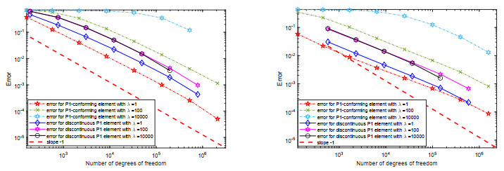
Example 4.1. We use Scheme 3.1 to compute the approximation for the 1st eigenvalue $\kappa_1$ of the problem (2.2). We adopt piecewise polynomial of degree 1 ($P1$ element) to compute on uniform isosceles right triangulations. We produce the initial coarse grid $\mathcal{T}_{H} = \mathcal{T}_{h_0}$ and refine the coarse grid in a uniform way (each triangle is divided into four congruent triangles) repeatedly to obtain fine grids $\mathcal{T}_{h_i}, i = 1, 2, ..., l$. By using the basis functions of ${\boldsymbol {S}}^{H}$, the eigenvalue problem on the initial coarse grid in Step 1 of Scheme 3.1 can be rewritten as a generalized matrix eigenvalue problem

where the elements of array $\bar{\boldsymbol u}_{1, H}$ are the coordinates of $\boldsymbol u_{1, H}$ under the basis functions in ${\boldsymbol {S}}^{H}$. Similarly, by using the basis functions of ${\boldsymbol {S}}^{h_{i}}$, the algebraic system in Step 3 of Scheme 3.1 can be rewritten as

and $\bar{\boldsymbol u}_{1}^{h_{i}} = \frac{\hat{\boldsymbol u}}{\sqrt{\hat{\boldsymbol u}^T M^{h_{i}}\hat{\boldsymbol u}}}$ where $\hat{\boldsymbol u}_{1}^{h_{i-1}}$ is actually the projection of the solution $\bar{\boldsymbol u}_{1}^{h_{i-1}}$ obtained on the previous grid $\mathcal{T}_{h_{i-1}}$ in $\mathcal{T}_{h_{i}}$. For example, if $\mathcal{T}_{h_{0}}$ contains $NT = 2$ elements with the associated solution $\bar{{\boldsymbol u}}_1^{h_{0}} = \bar{\boldsymbol u}_{1, H}$, denote $\bar{{\boldsymbol u}}_{1}^{h_{0}} = [u_{1}^{h_{0}}, u_{2}^{h_{0}}]^T$ with $u_{1}^{h_{0}} = [a_{11}, a_{21}, a_{12}, a_{22}, a_{13}, a_{23}]$, $u_{2}^{h_{0}} = [b_{11}, b_{21}, b_{12}, b_{22}, b_{13}, b_{23}]$ and $a_{\iota j}, b_{\iota j}(j = 1, 2, 3)$ being the coordinates of the basis function $\{1, x, y\}$ on the element $\iota$ in $\mathcal{T}_{h_{0}}$, and encrypt $\mathcal{T}_{h_{0}}$ once (each triangle is divided into four congruent triangles) to get $\mathcal{T}_{h_{1}}$ which contains $4NT = 8$ elements, then the projection of $\bar{{\boldsymbol u}}_1^{h_{0}}$ in $\mathcal{T}_{h_{1}}$ is as follows:

where $Q_1$ is the projection (restriction) operator:

If bisecting encryption is used, that is, each triangle is divided into two triangles, then just replace $I_{NT}^4$ with $I_{NT}^2 = \left [ {\begin{array}{c} I_{NT} \\ I_{NT} \\ \end{array} } \right ]$. We use the command "${\mathtt{eigs}}$" of MATLAB to solve the discrete algebraic eigenvalue problem (4.1), and use the command "$\setminus$" in MATLAB to solve the linear system (4.2). Further, there has no difficulty with solving the system (4.2) (see Lecture 27.4 in ^[36]).

For comparison, we also use the multigrid method of conforming finite elements by adopting $P1$ element to compute. The error curves are depicted in Figure 1 where the reference value are taken as the most accurate approximations that we can compute. From Figure 1, we can see that as the Lamé parameter $\lambda$ increases, the DG-multigrid method is robust compared with the multigrid method of conforming finite elements, which is a major advantage of using DG method to solve elastic problems.

Example 4.2. Adaptive computation.

Adaptive algorithm based on the a posterior error estimation is an efficient and important numerical approach for solving partial differential equations. Referring to ^[37], we combine the multigrid scheme 3.1 and the a posteriori error indicator to establish the adaptive multigrid algorithm. Referring to the a posterior error indicator $(25)$ for the linear elastic source problem in ^[37], we formally give the following local error indicator for the underlying eigenvalue problem:

where

Define the global error indicator:

Based on the above error indicators and Scheme 3.1, we design the following adaptive multigrid algorithm bases on the shifted inverse iteration.

Algorithm 4.1. Choose parameter $0 < \alpha < 1$.

Step 1: Pick any initial mesh $\mathcal{T}_{h_0}$.

Step 2: Solve $(2.3)$ on $\mathcal{T}_{h_0}$ for discrete solution $(\kappa_{j, h_0}, {{\boldsymbol {u}}}_{j, h_0})$.

Step 3: Let $l = 1$. ${{\boldsymbol {u}}}_{j}^{h_1} \Leftarrow {{\boldsymbol {u}}}_{j, h_0}, \kappa_{j}^{h_1} \Leftarrow \kappa_{j, h_0}$.

Step 4: Compute the local indicator $\zeta_{K}(\kappa_{j}^{h_l}, {{\boldsymbol {u}}}_{j}^{h_l})$.

Step 5: Construct $\widehat{\mathcal{T}}_{h_l} \subset \ \mathcal{T}_{h_l}$ by Mark Strategy and parameter $\alpha$.

Step 6: Refine $\mathcal{T}_{h_l}$ to get a new mesh $\mathcal{T}_{h_{l+1}}$ by procedure REFINE.

Step 7: Find ${\boldsymbol {\widetilde{u}}} \in {{\boldsymbol {S}}}^{h_{l+1}}$ such that

Denote ${{\boldsymbol {u}}}_{j}^{h_{l+1}} = \frac{{\boldsymbol {\widetilde{u}}}}{\| {\boldsymbol {\widetilde{u}}} \|_{0, \partial\Omega}}$ and compute the Rayleigh quotient

Step 8: Let $l = l+1$ and go to Step 4.

Mark Strategy

Given parameter $0 < \alpha < 1$.

Step 1: Construct a minimal subset $\widehat{\mathcal{T}}_{h_{l}}$ of $\mathcal{T}_{h_{l}}$ by selecting some elements in $\mathcal{T}_{h_{l}}$ such that

Step 2: Mark all elements in $\widehat{\mathcal{T}}_{h_{l}}$.

Mark Strategy was first proposed in ^[38], and the procedure REFINE is some iterative or recursive bisection (see, e.g., ^[39,40]) of elements with the minimal refinement condition that marked elements are bisected at least once.

In addition, to investigate the efficiency of Algorithm 4.1, referring to the standard popular adaptive algorithm ^[41] we give the following Algorithm 4.2 for comparison.

Algorithm 4.2. Choose parameter $0 < \alpha < 1$.

Step 1: Pick any initial mesh $\mathcal{T}_{h_0}$.

Step 2: Solve (2.3) on $\mathcal{T}_{h_0}$ for discrete solution $(\kappa_{j, h_1}, {{\boldsymbol {u}}}_{j, h_1})$.

Step 3: Let $l = 1$.

Step 4: Compute the local indicators $\zeta_{K}(\kappa_{j, h_l}, {{\boldsymbol {u}}}_{j, h_l})$.

Step 5: Construct $\widehat{\mathcal{T}}_{h_l} \subset \ \mathcal{T}_{h_l}$ by Mark Strategy and parameter $\alpha$.

Step 6: Refine $\mathcal{T}_{h_l}$ to get a new mesh $\mathcal{T}_{h_{l+1}}$ by procedure REFINE.

Step 7: Solve (2.3) on $\mathcal{T}_{h_{l+1}}$ for discrete solution $(\kappa_{j, h_{l+1}}, {{\boldsymbol {u}}}_{j, h_{l+1}})$.

Step 8: Let $l = l+1$ and go to Step 4.

We use the adaptive DG-multigrid method (Algorithm 4.1) with polynomials of degree 1 ($P1$ element) and degree 2 ($P2$ element) to compute, and take $\alpha = 0.5$. For convenience of reading, we specify the following notations in our tables and figures.

$-$ $N_{j, l}$: the degrees of freedom at the $l$th iteration;

$-$ $\kappa_{j}^{h_l}$: the $j$th eigenvalue obtained by Algorithm 4.1 at the $\ l \ $th iteration;

$-$ $\kappa_{j, h_l}$: the $j$th eigenvalue obtained by Algorithm 4.2 at the $\ l \ $th iteration;

$-$ $CPU_{j, l}(s)$: the CPU time(s) from the first iteration beginning to the calculate results of the $l$th iteration appearing by using Algorithm 4.1/4.2;

$-$ $e_j$: the error of the $j$th approximate eigenvalue by Algorithm 4.1;

$-$ $\zeta_j$: the error indicator of the $j$th approximate eigenvalue by Algorithm 4.1.

We first give a numerical experiment comparison between using DGFEM to solve directly on fine meshes and using the adaptive DG-multigrid method (Algorithm 4.1) for the 1st nonzero eigenvalue of (2.3). The error curves are shown in Figures 2 and 3. An observation of the left and right subgraphs in Figures 2 and 3 tells us that the regularity of the eigenfunction in $\Omega_L$ is lower than that in $\Omega_S$, which is consistent with the general conclusion of the regularity of solutions to PDEs. From Figure 2 we can see that the error curves of adaptive DG-multigrid method are all parallel to the line with slope $-1$ but the error curves of directly computing by DGFEM do not parallel, which indicates that the approximate eigenvalues obtained by the adaptive DG-multigrid method achieve the optimal convergence order. The same conclusion can be seen from Figure 3.

Now we use Algorithms 4.1 and 4.2 with $P1$ and $P2$ elements to compute the first 7 non-zero eigenvalues of (2.3) in $\Omega_S$ and $\Omega_L$, respectively. When using $P1$ element, the parameters $\mu = 1, \lambda = 1, \gamma_\mu = \gamma_\lambda = 10$ and the diameter of initial mesh is taken as $\frac{\sqrt{2}}{16}$. Limited to space, we list the 1st, the 3rd, the 4th and the 6th approximate eigenvalue in Tables 1 and 2. We also depict the error curves of approximate eigenvalues by Algorithm 4.1 and the curve of error indicators in Figure 4, where the reference values are taken as the most accurate approximations that we can compute. In addition, for the 1st non-zero eigenvalue of (2.3), we investigate the influence of Lamé parameter by taking $\lambda = 1, 10,100, 1000, 10000$, and the corresponding error curves are shown in Figure 5. When using $P2$ element, the parameters $\mu = \lambda = 1, \gamma_\mu = \gamma_\lambda = 40$ and the diameter of initial mesh is taken as $\frac{\sqrt{2}}{8}$. In Tables 3 and 4 we list the 1st, the 3rd, the 4th and the 6th approximate eigenvalue. We also plot the error curves of approximate eigenvalues by Algorithm 4.1 and the curve of error indicators in Figure 6. For the 1st non-zero eigenvalue of (2.3), we investigate the influence of Lamé parameter by taking $\lambda = 1, 10,100, 1000, 10000$, and the corresponding error curves are shown in Figure 7.

It can be seen from Tables 1–4 that to get the same accurate approximate eigenvalues, Algorithm 4.1 uses less time or less degrees of freedom than Algorithm 4.2. In Figure 4, the error curves $e_1, e_3, e_4$ and $e_6$ are all parallel to the line with slope $-1$, and in Figure 6 the error curves $e_1, e_3, e_4$ and $e_6$ are parallel to the line with slope $-2$, which indicate that the approximate eigenvalues obtained by Algorithm 4.1 achieve the optimal convergence order. Meanwhile, in Figure 5, the error curves $e_1, e_3, e_4$ and $e_6$ are almost parallel to the curve of $\zeta_1, \zeta_3, \zeta_4$ and $\zeta_6$ respectively, and in Figure 7, the curves of $e_1, e_3, e_4$ and $e_6$ are parallel to $\zeta_1, \zeta_3, \zeta_4$ and $\zeta_6$, which indicate that the error indicators are reliable and efficient. Figures 5 and 7 then show that Algorithm 4.1 is robust in both $\Omega_S$ and $\Omega_L$.

5.   Conclusions

In this paper, we discussed a multigrid discretization scheme of DGFEM based on the shifted-inverse iteration. Theoretical analysis and numerical results all showed that this method can efficiently solve the Steklov-Lamé eigenproblem as we expected. Generally, the time of solving a linear algebraic system is much less than that of solving an eigenvalue problem. Further, we observe from Tables 1–4 that although the CPU time of the adaptive DG-multigrid method is less than that of the standard adaptive DGFEM, the advantage is not obvious. We think that this may be because we use "$\setminus$" to solve linear algebraic systems. We notice that in recent research, the multigrid method has been combined with other methods to form many efficient algorithms and applied to many problems, as combined with the DG method in this paper. For example, the multigrid-homotopy method to diffusion equation ^[42], the multigrid method for the semilinear interface problem based on the modified two-grid method ^[43], the multigrid method for nonlinear eigenvalue problems based on Newton iteration ^[44], etc. It is of interest for us to explore more applications of multigrid methods and more efficient solvers for solving linear algebraic equations in multigrid methods.

Acknowledgments

This work was supported by the National Natural Science Foundation of China (No. 12261024) and Science and Technology Planning Project of Guizhou Province (Guizhou Kehe fundamental research-ZK[2022] No.324).

Conflict of interest

This work does not have any conflicts of interest.