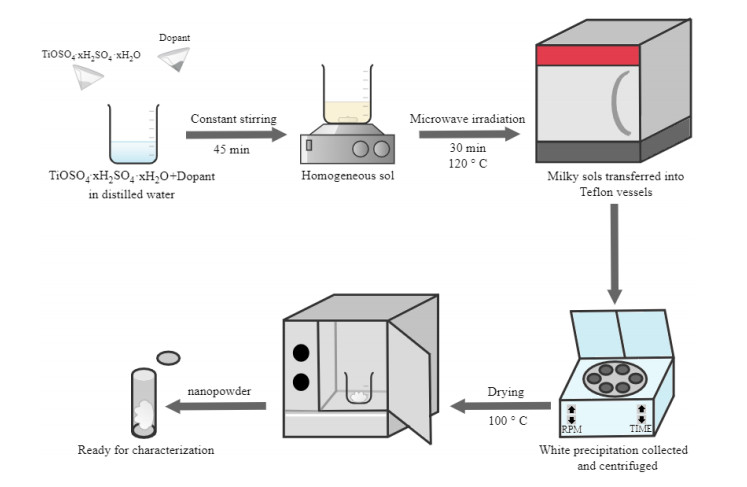
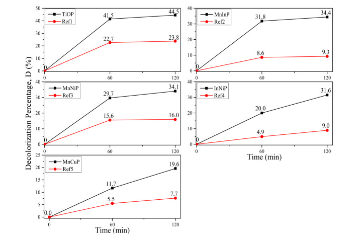
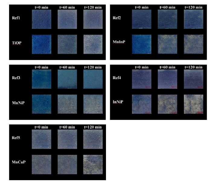
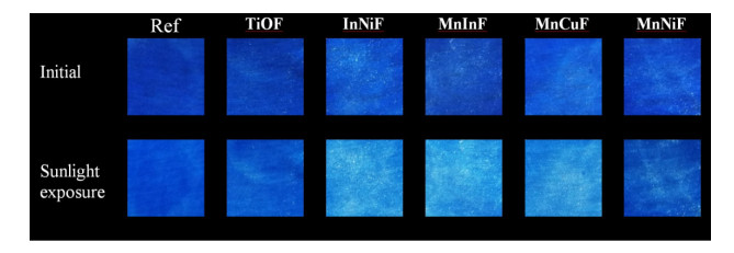
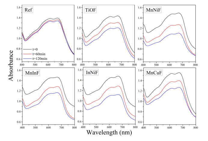
Nanostructured titanium dioxide (TiO2) among other oxides can be used as a prominent photocatalytic nanomaterial with self-cleaning properties. TiO2 is selected in this research, due to its high photocatalytic activity, high stability and low cost. Metal doping has proved to be a successful approach for enhancing the photocatalytic efficiency of photocatalysts. Photocatalytic products can be applied in the building sector, using both building materials as a matrix, but also in fabrics. In this study undoped and Mn-In, Mn-Cu, In-Ni, Mn-Ni bimetallic doped TiO2 nanostructures were synthesized using the microwave-assisted hydrothermal method. Decolorization efficiency of applied nanocoatings on fabrics and 3-D printed sustainable blocks made from recycled building materials was studied, both under UV as well as visible light for Methylene Blue (MB), using a self-made depollution and self-cleaning apparatus. Nanocoated samples showed high MB decolorization and great potential in self-cleaning applications. Results showed that the highest MB decolorization for both applications were observed for 0.25 at% Mn-In doped TiO2. For the application of 3-D printed blocks Mn-In and In-Ni doped TiO2 showed the highest net MB decolorization, 25.1 and 22.6%, respectively. For the application of nanocoated fabrics, three samples (Mn-In, In-Ni and Mn-Cu doped TiO2) showed high MB decolorization (58.1, 52.7 and 47.6%, respectively) under indirect sunlight, while under UV light the fabric coated with Mn-In and In-Ni doped TiO2 showed the highest MB decolorization rate 26.1 and 24.0%, respectively.
Citation: Evangelos Karagiannis, Dimitra Papadaki, Margarita N. Assimakopoulos. Circular self-cleaning building materials and fabrics using dual doped TiO2 nanomaterials[J]. AIMS Materials Science, 2022, 9(4): 534-553. doi: 10.3934/matersci.2022032
Nanostructured titanium dioxide (TiO2) among other oxides can be used as a prominent photocatalytic nanomaterial with self-cleaning properties. TiO2 is selected in this research, due to its high photocatalytic activity, high stability and low cost. Metal doping has proved to be a successful approach for enhancing the photocatalytic efficiency of photocatalysts. Photocatalytic products can be applied in the building sector, using both building materials as a matrix, but also in fabrics. In this study undoped and Mn-In, Mn-Cu, In-Ni, Mn-Ni bimetallic doped TiO2 nanostructures were synthesized using the microwave-assisted hydrothermal method. Decolorization efficiency of applied nanocoatings on fabrics and 3-D printed sustainable blocks made from recycled building materials was studied, both under UV as well as visible light for Methylene Blue (MB), using a self-made depollution and self-cleaning apparatus. Nanocoated samples showed high MB decolorization and great potential in self-cleaning applications. Results showed that the highest MB decolorization for both applications were observed for 0.25 at% Mn-In doped TiO2. For the application of 3-D printed blocks Mn-In and In-Ni doped TiO2 showed the highest net MB decolorization, 25.1 and 22.6%, respectively. For the application of nanocoated fabrics, three samples (Mn-In, In-Ni and Mn-Cu doped TiO2) showed high MB decolorization (58.1, 52.7 and 47.6%, respectively) under indirect sunlight, while under UV light the fabric coated with Mn-In and In-Ni doped TiO2 showed the highest MB decolorization rate 26.1 and 24.0%, respectively.

| [1] | Papadaki D, Kiriakidis G, Tsoutsos T (2018) Applications of nanotechnology in construction industry, In: Barhoum A, Abdel Salam HM, Fundamentals of Nanoparticles, Elsevier, 343-370. https://doi.org/10.1016/B978-0-323-51255-8.00011-2 |
| [2] |
Boostani H, Modirrousta S (2016) Review of nanocoatings for building application. Procedia Eng 145: 1541-1548. https://doi.org/10.1016/j.proeng.2016.04.194 doi: 10.1016/j.proeng.2016.04.194

|
| [3] |
Jesus MAMLD, Neto JTDS, Timò G, et al. (2015) Superhydrophilic self-cleaning surfaces based on TiO2 and TiO2/SiO2 composite films for photovoltaic module cover glass. Appl Adhes Sci 3: 5. https://doi.org/10.1186/s40563-015-0034-4 doi: 10.1186/s40563-015-0034-4
|
| [4] |
Luna M, Delgado J, Gil M, et al. (2018) TiO2-SiO2 coatings with a low content of AuNPs for producing self-cleaning building materials. Nanomaterials 8: 177. https://doi.org/10.3390/nano8030177 doi: 10.3390/nano8030177
|
| [5] |
Ünlü B, Özacar M (2020) Effect of Cu and Mn amounts doped to TiO2 on the performance of DSSCs. Sol Energy 196: 448-456. https://doi.org/10.1016/j.solener.2019.12.043 doi: 10.1016/j.solener.2019.12.043
|
| [6] |
Papadaki D, Foteinis S, Binas V, et al. (2019) A life cycle assessment of PCM and VIP in warm Mediterranean climates and their introduction as a strategy to promote energy savings and mitigate carbon emissions. AIMS Mater Sci 6: 944-959. https://doi.org/10.3934/matersci.2019.6.944 doi: 10.3934/matersci.2019.6.944
|
| [7] |
Tisov A, Kuusk K, Escudero MN, et al. (2020) Driving decarbonisation of the EU building stock by enhancing a consumer centred and locally based circular renovation process. E3S Web of Conferences 172: 18006. https://doi.org/10.1051/e3sconf/202017218006 doi: 10.1051/e3sconf/202017218006
|
| [8] | Cheshire D (2019) Building Revolutions: Applying the Circular Economy to the Built Environment, RIBA Publishing. https://doi.org/10.4324/9780429346712 |
| [9] |
Mangialardo A, Micelli E (2018) Rethinking the construction industry under the circular economy: Principles and case studies. International conference on Smart and Sustainable Planning for Cities and Regions, 333-344. https://doi.org/10.1007/978-3-319-75774-2_23 doi: 10.1007/978-3-319-75774-2_23
|
| [10] |
Gao W, Zhang Y, Ramanujan D, et al. (2015) The status, challenges, and future of additive manufacturing in engineering. Comput Aided Design 69: 65-89. https://doi.org/10.1016/j.cad.2015.04.001 doi: 10.1016/j.cad.2015.04.001
|
| [11] |
Xia M, Sanjayan J (2016) Method of formulating geopolymer for 3D printing for construction applications. Mater Design 110: 382-390. https://doi.org/10.1016/j.matdes.2016.07.136 doi: 10.1016/j.matdes.2016.07.136
|
| [12] |
Wangler T, Lloret E, Reiter L, et al. (2016) Digital Concrete: Opportunities and Challenges. RILEM Tech Lett 1: 67. https://doi.org/10.21809/rilemtechlett.2016.16 doi: 10.21809/rilemtechlett.2016.16
|
| [13] |
Mansour AMH, Al-Dawery SK (2018) Sustainable self-cleaning treatments for architectural facades in developing countries. Alex Eng J 57: 867-873. https://doi.org/10.1016/j.aej.2017.01.042 doi: 10.1016/j.aej.2017.01.042
|
| [14] |
Li Y (2019) Study on the weathering mechanism and protection technology of stone archives. IOP Conf Ser Mater Sci Eng 490: 062032. https://doi.org/10.1088/1757-899X/490/6/062032 doi: 10.1088/1757-899X/490/6/062032
|
| [15] | Janus M, Zając K (2019) Self-cleaning efficiency of nanoparticles applied on facade bricks, In: Pacheco-Torgal F, Diamanti MV, Nazari A, et al., Nanotechnology in Eco-efficient Construction: Materials, Processes and Applications, 2Eds., Elsevier, 591-618. https://doi.org/10.1016/B978-0-08-102641-0.00024-4 |
| [16] | Diamanti MV, Pedeferri M (2019) Photocatalytic performance of mortars with nanoparticles exposed to the urban environment, In: Pacheco-Torgal F, Diamanti MV, Nazari A, et al., Nanotechnology in Eco-efficient Construction: Materials, Processes and Applications, 2Eds., Elsevier, 527-555. https://doi.org/10.1016/B978-0-08-102641-0.00022-0 |
| [17] |
Sikora P, Horszczaruk E, Rucinska T (2015) The effect of nanosilica and titanium dioxide on the mechanical and self-cleaning properties of waste-glass cement mortar. Procedia Eng 108: 146-153. https://doi.org/10.1016/j.proeng.2015.06.130 doi: 10.1016/j.proeng.2015.06.130
|
| [18] |
Abbas M, Iftikhar H, Malik M, et al. (2018) Surface coatings of TiO2 nanoparticles onto the designed fabrics for enhanced self-cleaning properties. Coatings 8: 35. https://doi.org/10.3390/coatings8010035 doi: 10.3390/coatings8010035
|
| [19] |
Giesz P, Celichowski G, Puchowicz D, et al. (2016) Microwave-assisted TiO2: anatase formation on cotton and viscose fabric surfaces. Cellulose 23: 2143-2159. https://doi.org/10.1007/s10570-016-0916-z doi: 10.1007/s10570-016-0916-z
|
| [20] |
Humayun M, Raziq F, Khan A, et al. (2018) Modification strategies of TiO2 for potential applications in photocatalysis: a critical review. Green Chem Letter Rev 11: 86-102. https://doi.org/10.1080/17518253.2018.1440324 doi: 10.1080/17518253.2018.1440324
|
| [21] |
Nurdin M, Ramadhan LOAN, Darmawati D, et al. (2018) Synthesis of Ni, N co-doped TiO2 using microwave-assisted method for sodium lauryl sulfate degradation by photocatalyst. J Coat Technol Res 15: 395-402. https://doi.org/10.1007/s11998-017-9976-8 doi: 10.1007/s11998-017-9976-8
|
| [22] | Moma J, Baloyi J (2019) Modified titanium dioxide for photocatalytic applications, In: Khan SB, Akhta K, Photocatalysts: Applications and Attributes, IntechOpen. https://doi.org/10.5772/intechopen.79374 |
| [23] |
Maragatha J, Rajendran S, Endo T, et al. (2017) Microwave synthesis of metal doped TiO2 for photocatalytic applications. J Mater Sci-Mater El 28: 5281-5287. https://doi.org/10.1007/s10854-016-6185-7 doi: 10.1007/s10854-016-6185-7
|
| [24] |
Singh I, Birajdar B (2017) Synthesis, characterization and photocatalytic activity of mesoporous Na-doped TiO2 nano-powder prepared via a solvent-controlled non-aqueous sol-gel route. RSC Adv 7: 54053-54062. https://doi.org/10.1039/C7RA10108B doi: 10.1039/C7RA10108B
|
| [25] |
Qi H, Lee J, Wang L, et al. (2016) Photocatalytic performance of titanium dioxide nanoparticles doped with multi-metals. J Adv Oxid Technol 19: 302-309. https://doi.org/10.1515/jaots-2016-0214 doi: 10.1515/jaots-2016-0214
|
| [26] |
Gnanaprakasam A, Sivakumar VM, Thirumarimurugan M (2015) Influencing parameters in the photocatalytic degradation of organic effluent via nanometal oxide catalyst: A review. Indian J Mater Sci 2015: 1-16. https://doi.org/10.1155/2015/601827 doi: 10.1155/2015/601827
|
| [27] |
Colangiuli D, Calia A, Bianco N (2015) Novel multifunctional coatings with photocatalytic and hydrophobic properties for the preservation of the stone building heritage. Constr Build Mater 93: 189-196. https://doi.org/10.1016/j.conbuildmat.2015.05.100 doi: 10.1016/j.conbuildmat.2015.05.100
|
| [28] | Matoh L, Žener B, Korošec RC, et al. (2019) Photocatalytic water treatment, In: Pacheco-Torgal F, Diamanti MV, Nazari A, et al., Nanotechnology in Eco-efficient Construction: Materials, Processes and Applications, 2Eds., Elsevier, 675-702. https://doi.org/10.1016/B978-0-08-102641-0.00027-X |
| [29] | Janjua ZA (2019) Icephobic nanocoatings for infrastructure protection, In: Pacheco-Torgal F, Diamanti MV, Nazari A, et al., Nanotechnology in Eco-efficient Construction: Materials, Processes and Applications, 2Eds., Elsevier, 281-302. https://doi.org/10.1016/B978-0-08-102641-0.00013-X |
| [30] |
Bai W, Tian X, Yao R, et al. (2020) Preparation of nano-TiO2@polyfluorene composite particles for the photocatalytic degradation of organic pollutants under sunlight. Sol Energy 196: 616-624. https://doi.org/10.1016/j.solener.2019.12.066 doi: 10.1016/j.solener.2019.12.066
|
| [31] |
Bai W, Yao R, Tian X, et al. (2018) Sunlight highly photoactive TiO2@poly-p-phenylene composite microspheres for malachite green degradation. J Taiwan Inst Chem E 87: 112-116. https://doi.org/10.1016/j.jtice.2018.03.018 doi: 10.1016/j.jtice.2018.03.018
|
| [32] |
Colomer MT, Roa C, Ortiz AL, et al. (2020) Influence of Nd3+ doping on the structure, thermal evolution and photoluminescence properties of nanoparticulate TiO2 xerogels. J Alloy Compd 819: 152972. https://doi.org/10.1016/j.jallcom.2019.152972 doi: 10.1016/j.jallcom.2019.152972
|
| [33] |
Pipil H, Yadav S, Chawla H, et al. (2022) Comparison of TiO2 catalysis and Fenton's treatment for rapid degradation of Remazol Red Dye in textile industry effluent. Rend Lincei-Sci Fis 33: 105-114. https://doi.org/10.1007/s12210-021-01040-x doi: 10.1007/s12210-021-01040-x
|
| [34] |
Anucha CB, Altin I, Bacaksiz E, et al. (2022) Titanium dioxide (TiO2)-based photocatalyst materials activity enhancement for contaminants of emerging concern (CECs) degradation: In the light of modification strategies. Chem Eng J Adv 10: 100262. https://doi.org/10.1016/j.ceja.2022.100262 doi: 10.1016/j.ceja.2022.100262
|
| [35] |
Dharma HNC, Jaafar J, Widiastuti N, et al. (2022) A review of titanium dioxide (TiO2)-based photocatalyst for oilfield-produced water treatment. Membranes 12: 345. https://doi.org/10.3390/membranes12030345 doi: 10.3390/membranes12030345
|
| [36] |
Shimi AK, Ahmed HM, Wahab M, et al. (2022) Synthesis and applications of green synthesized TiO2 nanoparticles for photocatalytic dye degradation and antibacterial activity. J Nanomater 2022: 1-9. https://doi.org/10.1155/2022/7060388 doi: 10.1155/2022/7060388
|
| [37] |
Bregadiolli BA, Fernandes SL, Graeff CFDO (2017) Easy and fast preparation of TiO2-based nanostructures using microwave assisted hydrothermal synthesis. Mater Res 20: 912-919. https://doi.org/10.1590/1980-5373-mr-2016-0684 doi: 10.1590/1980-5373-mr-2016-0684
|
| [38] |
Dhilip Kumar R, Andou Y, Sathish M, et al. (2016) Synthesis of nanostructured Cu-WO3 and CuWO4 for supercapacitor applications. J Mater Sci-Mater El 27: 2926-2932. https://doi.org/10.1007/s10854-015-4111-z doi: 10.1007/s10854-015-4111-z
|
| [39] |
Jaafar NF, Marfur NA, Jusoh NWC, et al. (2019) Synthesis of mesoporous nanoparticles via microwave-assisted method for photocatalytic degradation of phenol derivatives. Malaysian J Anal Sci 23: 462-471. https://doi.org/10.17576/mjas-2019-2303-10 doi: 10.17576/mjas-2019-2303-10
|
| [40] | Rohrer GS (2001) Structure and Bonding in Crystalline Materials, Cambridge University Press. https://doi.org/10.1017/CBO9780511816116 |
| [41] | Pauling L (1960) The nature of the chemical bond and the structure of molecules and crystals: An introduction to modern structural chemistry, George Fisher Baker nonresident lectureship in chemistry at Cornell University, 3 Eds., Ithaca: Cornell University Press. |
| [42] | Galasso FS (1970) Structure and properties of inorganic solids, In: Francis S. Galasso. Illustrated by W. Darby. Pergamon Press Oxford, New York, 1st ed edition. |
| [43] |
Papadaki D, Mhlongo GH, Motaung DE, et al. (2019) Hierarchically porous Cu-, Co-, and Mn-doped platelet-like ZnO nanostructures and their photocatalytic performance for indoor air quality control. ACS Omega 4: 16429-16440. https://doi.org/10.1021/acsomega.9b02016 doi: 10.1021/acsomega.9b02016
|
| [44] |
Amreetha S, Dhanuskodi S, Nithya A, et al. (2016) Three way electron transfer of a C-N-S tri doped two-phase junction of TiO2 nanoparticles for efficient visible light photocatalytic dye degradation. RSC Adv 6: 7854-7863. https://doi.org/10.1039/C5RA25017J doi: 10.1039/C5RA25017J
|
| [45] |
Belekbir S, el Azzouzi M, el Hamidi A, et al. (2020) Improved photocatalyzed degradation of phenol, as a model pollutant, over metal-impregnated nanosized TiO2. Nanomaterials 10: 996. https://doi.org/10.3390/nano10050996 doi: 10.3390/nano10050996
|
| [46] |
Wilson GJ, Matijasevich AS, Mitchell DRG, et al. (2006) Modification of TiO2 for enhanced surface properties: Finite ostwald ripening by a microwave hydrothermal process. Langmuir 22: 2016-2027. https://doi.org/10.1021/la052716j doi: 10.1021/la052716j
|
| [47] |
El Mragui A, Logvina Y, Pinto da Silva L, et al. (2019) Synthesis of Fe- and Co-doped TiO2 with improved photocatalytic activity under visible irradiation toward carbamazepine degradation. Materials 12: 3874. https://doi.org/10.3390/ma12233874 doi: 10.3390/ma12233874
|
| [48] |
Irfan H, Racik KM, Anand S (2018) Microstructural evaluation of CoAl2O4 nanoparticles by Williamson-Hall and size-strain plot methods. J Asian Ceram Soc 6: 54-62. https://doi.org/10.1080/21870764.2018.1439606 doi: 10.1080/21870764.2018.1439606
|
| [49] |
Ghasemifard M, Abrishami ME, Iziy M (2015) Effect of different dopants Ba and Ag on the properties of SrTiO3 nanopowders. Result Phys 5: 309-313. https://doi.org/10.1016/j.rinp.2015.10.005 doi: 10.1016/j.rinp.2015.10.005
|
| [50] |
Nath D, Singh F, Das R (2020) X-ray diffraction analysis by Williamson-Hall, Halder-Wagner and size-strain plot methods of CdSe nanoparticles-a comparative study. Mater Chem Phys 239: 122021. https://doi.org/10.1016/j.matchemphys.2019.122021 doi: 10.1016/j.matchemphys.2019.122021
|
| [51] |
Dey PCh, Sarkar S, Das R (2020) X-ray diffraction study of the elastic properties of jagged spherical CdS nanocrystals. Mater Sci-Poland 38: 271-278. https://doi.org/10.2478/msp-2020-0032 doi: 10.2478/msp-2020-0032
|
| [52] |
Rabiei M, Palevicius A, Monshi A, et al. (2020) Comparing methods for calculating nano crystal size of natural hydroxyapatite using X-ray diffraction. Nanomaterials 10: 1627. https://doi.org/10.3390/nano10091627 doi: 10.3390/nano10091627
|
| [53] |
Gao X, Zhou B, Yuan R (2015) Doping a metal (Ag, Al, Mn, Ni and Zn) on TiO2 nanotubes and its effect on Rhodamine B photocatalytic oxidation. Environ Eng Res 20: 329-335. https://doi.org/10.4491/eer.2015.062 doi: 10.4491/eer.2015.062
|
| [54] |
Lee H-M, Kang H-R, An K-H, et al. (2013) Comparative studies of porous carbon nanofibers by various activation methods. Carbon Lett 14: 180-185. https://doi.org/10.5714/CL.2013.14.3.180 doi: 10.5714/CL.2013.14.3.180
|
| [55] |
Moradi H, Eshaghi A, Hosseini SR, et al. (2016) Fabrication of Fe-doped TiO2 nanoparticles and investigation of photocatalytic decolorization of reactive red 198 under visible light irradiation. Ultrason Sonochem 32: 314-319. https://doi.org/10.1016/j.ultsonch.2016.03.025 doi: 10.1016/j.ultsonch.2016.03.025
|
| [56] |
Iqbal A, Ibrahim NH, Rahman NRA, et al. (2020) ZnO surface doping to enhance the photocatalytic activity of lithium titanate/TiO2 for methylene blue photodegradation under visible light irradiation. Surfaces 3: 301-318. https://doi.org/10.3390/surfaces3030022 doi: 10.3390/surfaces3030022
|
Figures(11) / Tables(6)

Evangelos Karagiannis, Dimitra Papadaki, Margarita N. Assimakopoulos. Circular self-cleaning building materials and fabrics using dual doped TiO2 nanomaterials[J]. AIMS Materials Science, 2022, 9(4): 534-553. doi: 10.3934/matersci.2022032


 DownLoad: