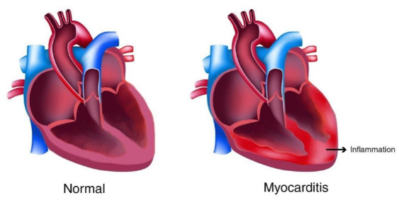
Myocarditis is the form of an inflammation of the middle layer of the heart wall which is caused by a viral infection and can affect the heart muscle and its electrical system. It has remained one of the most challenging diagnoses in cardiology. Myocardial is the prime cause of unexpected death in approximately 20% of adults less than 40 years of age. Cardiac MRI (CMR) has been considered a noninvasive and golden standard diagnostic tool for suspected myocarditis and plays an indispensable role in diagnosing various cardiac diseases. However, the performance of CMR depends heavily on the clinical presentation and features such as chest pain, arrhythmia, and heart failure. Besides, other imaging factors like artifacts, technical errors, pulse sequence, acquisition parameters, contrast agent dose, and more importantly qualitatively visual interpretation can affect the result of the diagnosis. This paper introduces a new deep learning-based model called Convolutional Neural Network-Clustering (CNN-KCL) to diagnose Myocarditis. In this study, we used 47 subjects with a total number of 98,898 images to diagnose myocarditis disease. Our results demonstrate that the proposed method achieves an accuracy of 97.41% based on 10 fold-cross validation technique with 4 clusters for diagnosis of Myocarditis. To the best of our knowledge, this research is the first to use deep learning algorithms for the diagnosis of myocarditis.
Citation: Danial Sharifrazi, Roohallah Alizadehsani, Javad Hassannataj Joloudari, Shahab S. Band, Sadiq Hussain, Zahra Alizadeh Sani, Fereshteh Hasanzadeh, Afshin Shoeibi, Abdollah Dehzangi, Mehdi Sookhak, Hamid Alinejad-Rokny. CNN-KCL: Automatic myocarditis diagnosis using convolutional neural network combined with k-means clustering[J]. Mathematical Biosciences and Engineering, 2022, 19(3): 2381-2402. doi: 10.3934/mbe.2022110
Myocarditis is the form of an inflammation of the middle layer of the heart wall which is caused by a viral infection and can affect the heart muscle and its electrical system. It has remained one of the most challenging diagnoses in cardiology. Myocardial is the prime cause of unexpected death in approximately 20% of adults less than 40 years of age. Cardiac MRI (CMR) has been considered a noninvasive and golden standard diagnostic tool for suspected myocarditis and plays an indispensable role in diagnosing various cardiac diseases. However, the performance of CMR depends heavily on the clinical presentation and features such as chest pain, arrhythmia, and heart failure. Besides, other imaging factors like artifacts, technical errors, pulse sequence, acquisition parameters, contrast agent dose, and more importantly qualitatively visual interpretation can affect the result of the diagnosis. This paper introduces a new deep learning-based model called Convolutional Neural Network-Clustering (CNN-KCL) to diagnose Myocarditis. In this study, we used 47 subjects with a total number of 98,898 images to diagnose myocarditis disease. Our results demonstrate that the proposed method achieves an accuracy of 97.41% based on 10 fold-cross validation technique with 4 clusters for diagnosis of Myocarditis. To the best of our knowledge, this research is the first to use deep learning algorithms for the diagnosis of myocarditis.

| [1] |
J. H. Joloudari, E. H. Joloudari, H. Saadatfar, M. Ghasemigol, S. M. Razavi, A. Mosavi, et al., Coronary artery disease dagnosis; ranking the significant features using a random trees model, Int. J. Environ. Res. Public Health, 17 (2020), 731. https://doi.org/10.3390/ijerph17030731. doi: 10.3390/ijerph17030731

|
| [2] | M. Aazam, E. N. Huh, Fog computing micro datacenter based dynamic resource estimation and pricing model for IoT, in 2015 IEEE 29th International Conference on Advanced Information Networking and Applications, IEEE, (2015), 687-694. https://doi.org/10.1109/AINA.2015.254. |
| [3] |
W. Cooper, S. Hernandez-Diaz, P. Arbogast, Myocarditis, N. Engl. J. Med., 354 (2006), 2443-2451. https://doi.org/10.1056/NEJMoa055202. doi: 10.1056/NEJMoa055202
|
| [4] |
L. A. Blauwet, L. T. Cooper, Myocarditis, Prog. Cardiovasc. Dis., 52 (2010), 274-288. https://doi.org/10.1016/j.pcad.2009.11.006. doi: 10.1016/j.pcad.2009.11.006
|
| [5] |
A. M. Feldman, D. McNamara, Myocarditis, N. Engl. J. Med., 343 (2000) 1388-1398. https://doi.org/10.1056/NEJM200011093431908. doi: 10.1056/NEJM200011093431908
|
| [6] |
R. Alizadehsani, M. H. Zangooei, M. J. Hosseini, J. Habibi, A. Khosravi, M. Roshanzamir, et al., Coronary artery disease detection using computational intelligence methods, Knowl. Based Syst., 109 (2016), 187-197. https://doi.org/10.1016/j.knosys.2016.07.004. doi: 10.1016/j.knosys.2016.07.004
|
| [7] |
E. Nasarian, M. Abdar, M. A. Fahami, R. Alizadehsani, S. Hussain, M. E. Basiri, et al., Association between work-related features and coronary artery disease: A heterogeneous hybrid feature selection integrated with balancing approach, Pattern Recognit. Lett., 133 (2020), 33-40. https://doi.org/10.1016/j.patrec.2020.02.010. doi: 10.1016/j.patrec.2020.02.010
|
| [8] |
R. Alizadehsani, M. Roshanzamir, M. Abdar, A. Beykikhoshk, A. Khosravi, S. Nahavandi, et al., Hybrid genetic-discretized algorithm to handle data uncertainty in diagnosing stenosis of coronary arteries, Expert Syst., 2020. https://doi.org/10.1111/exsy.12573. doi: 10.1111/exsy.12573
|
| [9] |
R. Alizadehsani, M. Roshanzamir, M. Abdar, A. Beykikhoshk, M. H. Zangooei, A. Khosravi, et al., Model uncertainty quantification for diagnosis of each main coronary artery stenosis, Soft Comput., 24 (2020) 10149-10160. https://doi.org/10.1007/s00500-019-04531-0. doi: 10.1007/s00500-019-04531-0
|
| [10] |
H. Greenspan, B. Van Ginneken, R. M. Summers, Guest editorial deep learning in medical imaging: overview and future promise of an exciting new technique, IEEE Trans. Med. Imaging, 35 (2016), 1153-1159. https://doi.org/10.1109/TMI.2016.2553401. doi: 10.1109/TMI.2016.2553401
|
| [11] |
B. Baeßler, M. Mannil, D. Maintz, H. Alkadhi, R. Manka, Texture analysis and machine learning of non-contrast T1-weighted MR images in patients with hypertrophic cardiomyopathy-Preliminary results, Eur. J. Radiol., 102 (2018), 61-67. https://doi.org/10.1016/j.ejrad.2018.03.013. doi: 10.1016/j.ejrad.2018.03.013
|
| [12] | M. Ovreiu, D. Simon, Biogeography-based optimization of neuro-fuzzy system parameters for diagnosis of cardiac disease, in Proceedings of the 12th Annual Conference on Genetic and Evolutionary Computation, (2010), 1235-1242. https://doi.org/10.1145/1830483.1830706. |
| [13] | M. Ali, M. F. Rani, A. H. Jahidin, M. F. Saaid, M. Z. H. Noor, Identification of cardiomyopathy disease using hybrid multilayered perceptron network, in 2012 IEEE International Conference on Control System, Computing and Engineering, IEEE, (2013), 23-27. https://doi.org/10.1109/ICCSCE.2012.6487109. |
| [14] |
D. Alis, A. Guler, M. Yergin, O. Asmakutlu, Assessment of ventricular tachyarrhythmia in patients with hypertrophic cardiomyopathy with machine learning-based texture analysis of late gadolinium enhancement cardiac MRI, Diagn. Interv. Imaging, 101 (2020), 137-146. https://doi.org/10.1016/j.diii.2019.10.005. doi: 10.1016/j.diii.2019.10.005
|
| [15] | S. Borkar, M. N. Annadate, Supervised machine learning algorithm for detection of cardiac disorders, in 2018 Fourth International Conference on Computing Communication Control and Automation (ICCUBEA), IEEE, (2018), 1-4.. https://doi.org/10.1109/ICCUBEA.2018.8697795. |
| [16] |
P. P. Sengupta, Y. M. Huang, M. Bansal, A. Ashrafi, M. Fisher, K. Shameer, et al., Cognitive machine-learning algorithm for cardiac imaging, Circ. Cardiovasc. Imaging, 9 (2016), e004330. https://doi.org/10.1161/CIRCIMAGING.115.004330. doi: 10.1161/CIRCIMAGING.115.004330
|
| [17] |
R. Begum, M. Ramesh, Detection of cardiomyopathy using support vector machine and artificial neural network, Int. J. Comput. Appl., 133 (2016), 29-34. https://doi.org/10.5120/ijca2016908178. doi: 10.5120/ijca2016908178
|
| [18] |
J. H. Joloudari, H. Saadatfar, A. Dehzangi, S. Shamshirband, Computer-aided decision-making for predicting liver disease using PSO-based optimized SVM with feature selection, Inf. Med. Unlocked, 17 (2019), 100255. https://doi.org/10.1016/j.imu.2019.100255. doi: 10.1016/j.imu.2019.100255
|
| [19] |
E. M. Green, R. Van Mourik, C. Wolfus, S. B. Heitner, O. Dur, M. J. Semigran, Machine learning detection of obstructive hypertrophic cardiomyopathy using a wearable biosensor, NPJ Digit. Med., 2 (2019), 57. https://doi.org/10.1038/s41746-019-0130-0. doi: 10.1038/s41746-019-0130-0
|
| [20] |
D. Y. Tsai, K. Kojima, Measurements of texture features of medical images and its application to computer-aided diagnosis in cardiomyopathy, Measurement, 37 (2005), 284-292. https://doi.org/10.1016/j.measurement.2004.11.015. doi: 10.1016/j.measurement.2004.11.015
|
| [21] |
S. Narula, K. Shameer, A. M. Salem Omar, J. T. Dudley, P. P. Sengupta, Machine-learning algorithms to automate morphological and functional assessments in 2D echocardiography, J. Am. Coll. Cardiol., 68 (2016), 2287. https://doi.org/10.1016/j.jacc.2016.08.062. doi: 10.1016/j.jacc.2016.08.062
|
| [22] |
Q. A. Rahman, L. G. Tereshchenko, M. Kongkatong, T. Abraham, M. R. Abraham, H. Shatkay, Utilizing ECG-based heartbeat classification for hypertrophic cardiomyopathy identification, IEEE Trans. Nanobiosci., 14 (2015), 505-512. https://doi.org/10.1109/TNB.2015.2426213. doi: 10.1109/TNB.2015.2426213
|
| [23] |
X. Shao, Y. Sun, K. Xiao, Y. Zhang, W. Zhang, Z. Kou, et al., Texture analysis of magnetic resonance T1 mapping with dilated cardiomyopathy: A machine learning approach, Medicine, 97 (2018), e12246. https://doi.org/10.1097/MD.0000000000012246. doi: 10.1097/MD.0000000000012246
|
| [24] |
G. Captur, W. Heywood, C. Coats, S. Rosmini, V. Patel, L. R. Lopes, et al., Identification of a multiplex biomarker panel for hypertrophic cardiomyopathy using quantitative proteomics and machine learning, Mol. Cell. Proteomics, 19 (2020), 114. https://doi.org/10.1074/mcp.RA119.001586. doi: 10.1074/mcp.RA119.001586
|
| [25] |
F. Ali, S. El-Sappagh, S. R. Islam, D. Kwak, A. Ali, M. Imran, et al., A smart healthcare monitoring system for heart disease prediction based on ensemble deep learning and feature fusion, Inf. Fusion, 63 (2020), 208-222. https://doi.org/10.1016/j.inffus.2020.06.008. doi: 10.1016/j.inffus.2020.06.008
|
| [26] |
A. Baccouche, B. Garcia-Zapirain, C. Castillo Olea, A. Elmaghraby, Ensemble deep learning models for heart disease classification: A case study from Mexico, Information, 11 (2020), 207. https://doi.org/10.3390/info11040207. doi: 10.3390/info11040207
|
| [27] | T. Chokwijitkul, A. Nguyen, H. Hassanzadeh, S. Perez, Identifying risk factors for heart disease in electronic medical records: A deep learning approach, in Proceedings of the BioNLP 2018 Workshop, (2018), 18-27. https://doi.org/10.18653/v1/W18-2303. |
| [28] |
Y. S. Su, T. J. Ding, M. Y. Chen, Deep learning methods in internet of medical things for valvular heart disease screening system, IEEE Internet Things J., 99 (2021), 1. https://doi.org/10.1109/JIOT.2021.3053420. doi: 10.1109/JIOT.2021.3053420
|
| [29] |
S. S. Sarmah, An efficient IoT-based patient monitoring and heart disease prediction system using deep learning modified neural network, IEEE Access, 8 (2020), 135784-135797. https://doi.org/10.1109/ACCESS.2020.3007561. doi: 10.1109/ACCESS.2020.3007561
|
| [30] |
S. A. Morris, K. N. Lopez, Deep learning for detecting congenital heart disease in the fetus, Nat. Med., 27 (2021), 764-765. https://doi.org/10.1038/s41591-021-01354-1. doi: 10.1038/s41591-021-01354-1
|
| [31] | S. Narmadha, S. Gokulan, M. Pavithra, R. Rajmohan, T. Ananthkumar, Determination of various deep learning parameters to predict heart disease for diabetes patients, in 2020 International Conference on System, Computation, Automation and Networking (ICSCAN), IEEE, (2020), 1-6. https://doi.org/10.1109/ICSCAN49426.2020.9262317. |
| [32] |
R. Bharti, A. Khamparia, M. Shabaz, G. Dhiman, S. Pande, P. Singh, Prediction of heart disease using a combination of machine learning and deep learning, Comput. Intell. Neurosci., 2021 (2021), 8387680. https://doi.org/10.1155/2021/8387680. doi: 10.1155/2021/8387680
|
| [33] |
J. M. Kwon, K. H. Kim, K. H. Jeon, J. Park, Deep learning for predicting in-hospital mortality among heart disease patients based on echocardiography, Echocardiography, 36 (2019), 213-218. https://doi.org/10.1111/echo.14220. doi: 10.1111/echo.14220
|
| [34] |
S. Sharma, M. Parmar, Heart diseases prediction using deep learning neural network model., Int. J. Innovative Technol. Explor. Eng., 9 (2020), 2278-3075. https://doi.org/10.35940/ijitee.C9009.019320. doi: 10.35940/ijitee.C9009.019320
|
| [35] |
R. Poplin, A. V. Varadarajan, K. Blumer, Y. Liu, M. V. McConnell, G. S. Corrado, et al., Prediction of cardiovascular risk factors from retinal fundus photographs via deep learning, Nat. Biomed. Eng., 2 (2018) 158-164. https://doi.org/10.1038/s41551-018-0195-0. doi: 10.1038/s41551-018-0195-0
|
| [36] |
M. Chetrit, M. G. Friedrich, The unique role of cardiovascular magnetic resonance imaging in acute myocarditis, F1000Research, 7 (2018), 1153. https://doi.org/10.12688/f1000research.14857.1. doi: 10.12688/f1000research.14857.1
|
| [37] |
M. D. Cornicelli, C. K. Rigsby, K. Rychlik, E. Pahl, J. D. Robinson, Diagnostic performance of cardiovascular magnetic resonance native T1 and T2 mapping in pediatric patients with acute myocarditis, J. Cardiovasc. Magn. Reson., 21 (2019), 40-48. https://doi.org/10.1186/s12968-019-0550-7. doi: 10.1186/s12968-019-0550-7
|
| [38] |
M. A. G. M. Olimulder, J. Van Es, M. A. Galjee, The importance of cardiac MRI as a diagnostic tool in viral myocarditis-induced cardiomyopathy, Neth. Heart J., 17 (2009), 481-486. https://doi.org/10.1007/BF03086308. doi: 10.1007/BF03086308
|
| [39] |
C. Moenninghoff, L. Umutlu, C. Kloeters, A. Ringelstein, M. E. Ladd, A. Sombetzki, et al., Workflow efficiency of two 1.5 T MR scanners with and without an automated user interface for head examinations, Acad. Radiol., 20 (2013), 721-730. https://doi.org/10.1016/j.acra.2013.01.004. doi: 10.1016/j.acra.2013.01.004
|
| [40] |
M. Khodatars, A. Shoeibi, N. Ghassemi, M. Jafari, A. Khadem, D. Sadeghi, et al., Deep learning for neuroimaging-based diagnosis and rehabilitation of autism spectrum disorder: a review, Comput. Biol. Med., 139 (2021). https://doi.org/10.1016/j.compbiomed.2021.104949. doi: 10.1016/j.compbiomed.2021.104949
|
| [41] |
N. Q. K. Le, Q. T. Ho, E. K. Y. Yapp, Y. Y. Ou, H. Y. Yeh, DeepETC: a deep convolutional neural network architecture for investigating and classifying electron transport chain's complexes, Neurocomputing, 375 (2020), 71-79. https://doi.org/10.1016/j.neucom.2019.09.070. doi: 10.1016/j.neucom.2019.09.070
|
| [42] |
J. N. Sua, S. Y. Lim, M. H. Yulius, X. Su, E. K. Y. Yapp, N. Q. K. Le, et al., Incorporating convolutional neural networks and sequence graph transform for identifying multilabel protein lysine ptm sites, Chemom. Intell. Lab. Syst., 206 (2020), 104171. https://doi.org/10.1016/j.chemolab.2020.104171. doi: 10.1016/j.chemolab.2020.104171
|
| [43] | N. Ghassemi, H. Mahami, M. T. Darbandi, A. Shoeibi, S. Hussain, F. Nasirzadeh, et al., Material recognition for automated progress monitoring using deep learning methods, preprint, arXiv: 2006.16344. |
| [44] |
A. Shoeibi, M. Khodatars, N. Ghassemi, M. Jafari, P. Moridian, R. Alizadehsani, et al., Epileptic seizure detection using deep learning techniques: a review, Int. J. Environ. Res. Public Health, 18 (2021), 5780. https://doi.org/10.3390/ijerph18115780. doi: 10.3390/ijerph18115780
|
| [45] |
L. Fu, B. Lu, B. Nie, Z. Peng, H. Liu, X. Pi, Hybrid network with attention mechanism for detection and location of myocardial infarction based on 12-lead electrocardiogram signals, Sensors, 20 (2020), 1020. https://doi.org/10.3390/s20041020. doi: 10.3390/s20041020
|
| [46] | Y. Le Cun, B. Boser, J. S. Denker, D. Henderson, R. E. Howard, W. Hubbard, et al., Handwritten digit recognition with a back-propagation network, in Proceedings of the 2nd International Conference on Neural Information Processing, (1990), 396-404. Available from: https://papers.nips.cc/paper/1989/file/53c3bce66e43be4f209556518c2fcb54-Paper.pdf. |
| [47] |
A. Krizhevsky, I. Sutskever, G. E. Hinton, Imagenet classification with deep convolutional neural networks, Adv. Neural Inf. Process. Syst., 25 (2012), 1097-1105. https://doi.org/10.1145/3065386. doi: 10.1145/3065386
|
| [48] | K. Simonyan, A. Zisserman, Very deep convolutional networks for large-scale image recognition, Comput. Sci., preprint, arXiv: 14091556. |
| [49] | C. Szegedy, W. Liu, Y. Jia, P. Sermanet, S. Reed, D. Anguelov, et al., Going deeper with convolutions; in 2015 IEEE Conference on Computer Vision and Pattern Recognition (CVPR), (2015), 1-9. https://doi.org/10.1109/CVPR.2015.7298594. |
| [50] | K. He, X. Zhang, S. Ren, J. Sun, Deep residual learning for image recognition, in 2016 IEEE Conference on Computer Vision and Pattern Recognition (CVPR), (2016), 770-778. https://doi.org/10.1109/CVPR.2016.90. |
| [51] |
S. Lawrence, C. L. Giles, T. Ah Chung, A. D. Back, Face recognition: a convolutional neural-network approach, IEEE Trans. Neural Networks, 8 (1997), 98-113. https://doi.org/10.1109/72.554195. doi: 10.1109/72.554195
|
| [52] |
R. Alizadehsani, M. Roshanzamir, S. Hussain, A. Khosravi, A. Koohestani, M. H. Zangooei, et al., Handling of uncertainty in medical data using machine learning and probability theory techniques: A review of 30 years (1991-2020), Ann. Oper. Res., (2021), 1-42. https://doi.org/10.1007/s10479-021-04006-2. doi: 10.1007/s10479-021-04006-2
|
| [53] |
H. Shin, H. R. Roth, M. Gao, L. Lu, Z. Xu, I. Nogues, et al., Deep convolutional neural networks for computer-aided detection: CNN architectures, dataset characteristics and transfer learning, IEEE Trans. Med. Imaging, 35 (2016), 1285-1298. https://doi.org/10.1109/TMI.2016.2528162. doi: 10.1109/TMI.2016.2528162
|
| [54] |
U. R. Acharya, H. Fujita, S. L. Oh, Y. Hagiwara, J. H. Tan, M. Adam, et al., Deep convolutional neural network for the automated diagnosis of congestive heart failure using ECG signals, Appl. Intell., 49 (2019), 16-27. https://doi.org/10.1007/s10489-018-1179-1. doi: 10.1007/s10489-018-1179-1
|
| [55] |
U. R. Acharya, H. Fujita, O. S. Lih, M. Adam, J. H. Tan, C. K. Chua, Automated detection of coronary artery disease using different durations of ECG segments with convolutional neural network, Knowl. Based Syst., 132 (2017), 62-71. https://doi.org/10.1016/j.knosys.2017.06.003. doi: 10.1016/j.knosys.2017.06.003
|
| [56] |
J. H. Tan, Y. Hagiwara, W. Pang, I. Lim, S. L. Oh, M. Adam, et al., Application of stacked convolutional and long short-term memory network for accurate identification of CADECG signals, Comput, Biol. Med., 94 (2018), 19-26. https://doi.org/10.1016/j.compbiomed.2017.12.023. doi: 10.1016/j.compbiomed.2017.12.023
|
| [57] |
A. Shoeibi, N. Ghassemi, R. Alizadehsani, M. Rouhani, H. Hosseini-Nejad, A. Khosravi, et al., A comprehensive comparison of handcrafted features and convolutional autoencoders for epileptic seizures detection in EEG signals, Expert Syst. Appl., 163 (2021), 113788. https://doi.org/10.1016/j.eswa.2020.113788. doi: 10.1016/j.eswa.2020.113788
|
| [58] | K. Wagstaff, C. Cardie, S. Rogers, S. Schrödl, Constrained k-means clustering with background knowledge, (2001), 577-584. Available from: http://www.litech.org/~wkiri/Papers/wagstaff-kmeans-01.pdf. |
| [59] |
A. K. Jain, Data clustering: 50 years beyond K-means, Pattern Recognit. Lett., 31 (2010), 651-666. https://doi.org/10.1016/j.patrec.2009.09.011. doi: 10.1016/j.patrec.2009.09.011
|
| [60] |
R. Alizadehsani, M. Roshanzamir, M. Abdar, A. Beykikhoshk, A. Khosravi, M. Panahiazar, et al., A database for using machine learning and data mining techniques for coronary artery disease diagnosis, Sci. Data, 6 (2019), 227. https://doi.org/10.1038/s41597-019-0206-3. doi: 10.1038/s41597-019-0206-3
|
| [61] |
G. Muhammad, M. S. Hossain, COVID-19 and non-COVID-19 classification using multi-layers fusion from lung ultrasound images, Inf. Fusion, 72 (2021), 80-88. https://doi.org/10.1016/j.inffus.2021.02.013. doi: 10.1016/j.inffus.2021.02.013
|
| [62] |
S. Hussain, G. Hazarika, Educational data mining model using rattle, Int. J. Adv. Comput. Sci. Appl., 5 (2014). https://doi.org/10.14569/IJACSA.2014.050605. doi: 10.14569/IJACSA.2014.050605
|
| [63] |
E. Haghighat, R. Juanes, Sciann: A keras/tensorflow wrapper for scientific computations and physics-informed deep learning using artificial neural networks, Comput. Methods Appl. Mech. Eng., 373 (2021), 113552. https://doi.org/10.1016/j.cma.2020.113552. doi: 10.1016/j.cma.2020.113552
|
| [64] |
R. Kumar, W. Wang, J. Kumar, T. Yang, A. Khan, W. Ali, et al., An integration of blockchain and AI for secure data sharing and detection of CT images for the hospitals, Comput. Med. Imaging Graph., 87 (2021), 101812. https://doi.org/10.1016/j.compmedimag.2020.101812. doi: 10.1016/j.compmedimag.2020.101812
|
| [65] |
R. Yamashita, J. Long, A. Saleem, D. L. Rubin, J. Shen, Deep learning predicts postsurgical recurrence of hepatocellular carcinoma from digital histopathologic images, Sci. Rep., 11 (2021), 2047. https://doi.org/10.1038/s41598-021-81506-y. doi: 10.1038/s41598-021-81506-y
|
| [66] | F. V. Jensen, F. Jensen, An introduction to Bayesian networks, Springer, 2014. https://doi.org/10.1007/978-3-642-54157-5_5. |
| [67] |
H. M. Afify, M. S. Zanaty, Computational predictions for protein sequences of COVID-19 virus via machine learning algorithms, Med. Biol. Eng. Comput., 59 (2021), 1723-1734. https://doi.org/10.21203/rs.3.rs-34004/v2. doi: 10.1007/s11517-021-02412-z
|
| [68] | F. Gorunescu, Data Mining: Concepts, models and techniques, Springer, 2011. https://doi.org/10.1007/978-3-642-19721-5. |
| [69] |
J. H. Joloudari, E. H. Joloudari, H. Saadatfar, M. GhasemiGol, S. M. Razavi, A. Mosavi, et al., Coronary artery disease diagnosis; ranking the significant features using a random trees model, Int. J. Environ. Res. Public Health, 17 (2020), 731. https://doi.org/10.3390/ijerph17030731. doi: 10.3390/ijerph17030731
|
| [70] |
I. Ruczinski, C. Kooperberg, M. LeBlanc, Logic regression, J. Comput. Graph. Stat., 12 (2003), 475-511. https://doi.org/10.1198/1061860032238. doi: 10.1198/1061860032238
|
| [71] |
G. Jones, J. Parr, P. Nithiarasu, S. Pant, A proof of concept study for machine learning application to stenosis detection, Med. Biol. Eng. Comput., 2021. https://doi.org/10.1007/s11517-021-02424-9. doi: 10.1007/s11517-021-02424-9
|
| [72] |
L. Breiman, Random forests, Mach. Learn., 45 (2001), 5-32. https://doi.org/10.1023/A:1010933404324. doi: 10.1023/A:1010933404324
|
| [73] |
I. Kindermann, C. Barth, F. Mahfoud, C. Ukena, M. Lenski, A. Yilmaz, et al., Update on myocarditis, J. Am. Coll. Cardiol., 59 (2012), 779. https://doi.org/10.1016/j.jacc.2011.09.074. doi: 10.1016/j.jacc.2011.09.074
|
| [74] |
T. S. Kafil, N. Tzemos, Myocarditis in 2020: advancements in imaging and clinical management, JACC Case Rep., 2 (2020), 178-179. https://doi.org/10.1016/j.jaccas.2020.01.004. doi: 10.1016/j.jaccas.2020.01.004
|
| [75] |
A. Roos, Diagnosis of myocarditis at cardiac MRI: the continuing quest for improved tissue characterization, Radiology, 292 (2019), 618-619. https://doi.org/10.1148/radiol.2019191476. doi: 10.1148/radiol.2019191476
|
| [76] |
F. Dominguez, U. Kühl, B. Pieske, P. Garcia-Pavia, C. Tschöpe, Update on myocarditis and inflammatory cardiomyopathy: reemergence of endomyocardial biopsy, Revista Española Cardiología, 69 (2016), 178-187. https://doi.org/10.1016/j.rec.2015.10.015. doi: 10.1016/j.rec.2015.10.015
|
| [77] |
C. Buttà, L. Zappia, G. Laterra, M. Roberto, Diagnostic and prognostic role of electrocardiogram in acute myocarditis: A comprehensive review, Ann. Noninvasive Electrocardiol., 1 (2020), 1-10. https://doi.org/10.1111/anec.12726. doi: 10.1111/anec.12726
|
| [78] |
P. Bholowalia, A. Kumar, EBK-means: A clustering technique based on elbow method and k-means in WSN, Int. J. Comput. Appl., 105 (2014), 17-24. https://doi.org/10.5120/18405-9674. doi: 10.5120/18405-9674
|


Figures(6) / Tables(7)

Danial Sharifrazi, Roohallah Alizadehsani, Javad Hassannataj Joloudari, Shahab S. Band, Sadiq Hussain, Zahra Alizadeh Sani, Fereshteh Hasanzadeh, Afshin Shoeibi, Abdollah Dehzangi, Mehdi Sookhak, Hamid Alinejad-Rokny. CNN-KCL: Automatic myocarditis diagnosis using convolutional neural network combined with k-means clustering[J]. Mathematical Biosciences and Engineering, 2022, 19(3): 2381-2402. doi: 10.3934/mbe.2022110


 DownLoad: