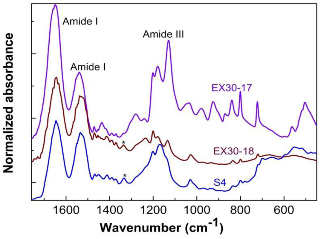
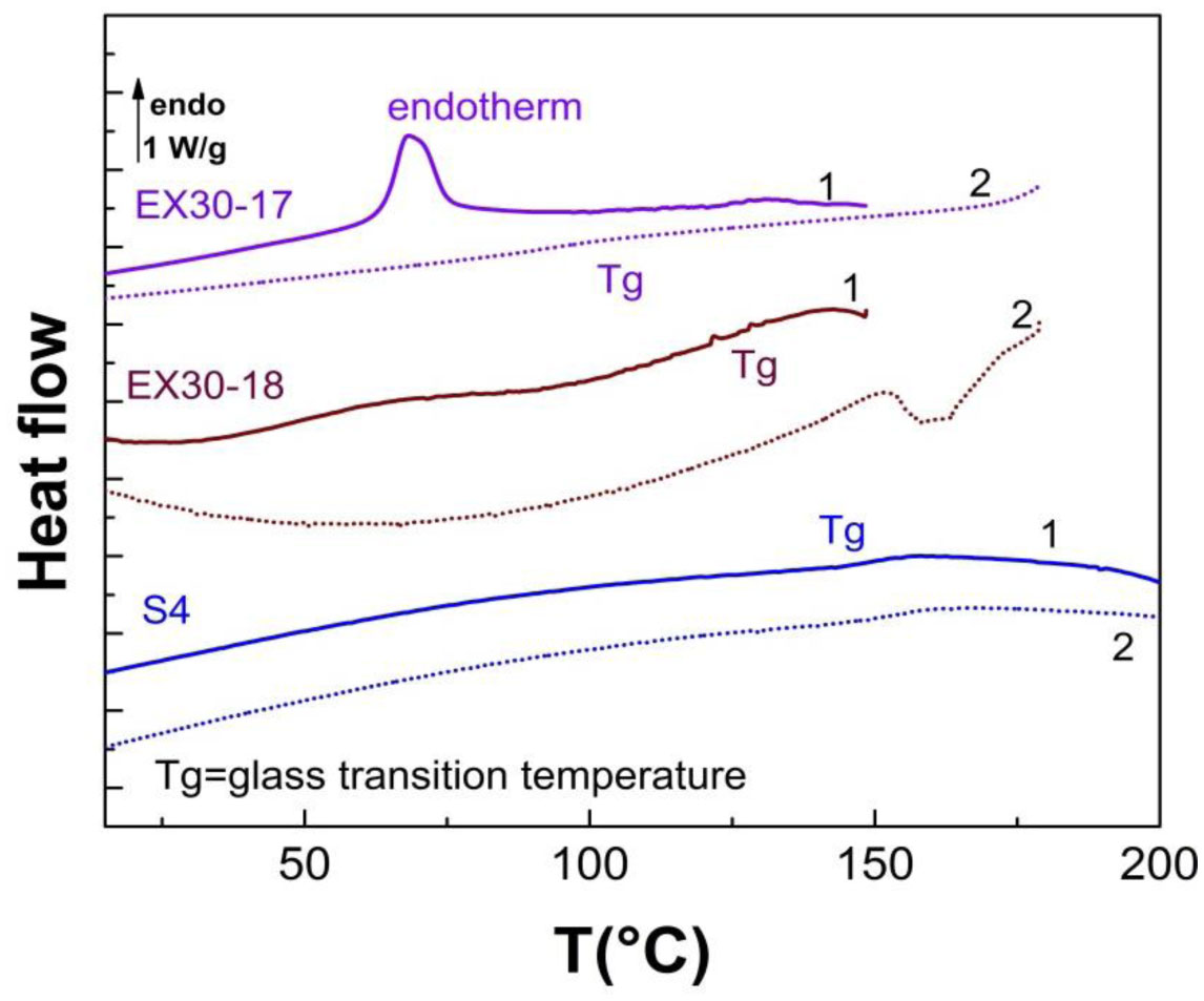
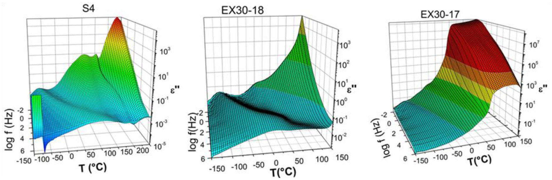
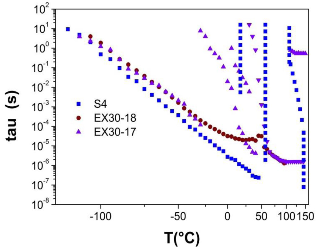
Three elastin peptides derived from a peculiar elastin sequence (exon 30) were investigated by Infra-red spectroscopy (IRTF), differential scanning calorimetry (DSC) and dielectric spectroscopy (DDS) to clarify the relationship between structural organization and physical properties of these peptides in the solid state. If a great majority of elastin derived peptides form organized structures, only few are able to coacervate, and only one, that is encoded by Exon 30, gives rise to an irreversible precipitation into amyloid fibers. The peptides studied in this work are constituted by 17, 18 or 22 amino acids whose sequences are contained in the longer exon 30. They all contain the XGGZG sequence (where X, Z = V, L) previously suspected to be responsible for amyloid formation in elastin peptides. Two of them gave rise to amyloid fibers while the other one was able to coacervate. In this work we attempted to correlate vibrational, thermal and dielectric behavior of these peptides in the solid state with the propensity to lead to reversible or irreversible aggregation in vivo.
Citation: J. Dandurand, E. Dantras, C. Lacabanne, A. Pepe, B. Bochicchio, V. Samouillan. Thermal and dielectric fingerprints of self-assembling elastin peptides derived from exon30[J]. AIMS Biophysics, 2021, 8(3): 236-247. doi: 10.3934/biophy.2021018
Three elastin peptides derived from a peculiar elastin sequence (exon 30) were investigated by Infra-red spectroscopy (IRTF), differential scanning calorimetry (DSC) and dielectric spectroscopy (DDS) to clarify the relationship between structural organization and physical properties of these peptides in the solid state. If a great majority of elastin derived peptides form organized structures, only few are able to coacervate, and only one, that is encoded by Exon 30, gives rise to an irreversible precipitation into amyloid fibers. The peptides studied in this work are constituted by 17, 18 or 22 amino acids whose sequences are contained in the longer exon 30. They all contain the XGGZG sequence (where X, Z = V, L) previously suspected to be responsible for amyloid formation in elastin peptides. Two of them gave rise to amyloid fibers while the other one was able to coacervate. In this work we attempted to correlate vibrational, thermal and dielectric behavior of these peptides in the solid state with the propensity to lead to reversible or irreversible aggregation in vivo.

| [1] |
Yeo GC, Keeley FW, Weiss AS (2011) Coacervation of tropoelastin. Adv Colloid Interfac Sci 167: 94-103. doi: 10.1016/j.cis.2010.10.003

|
| [2] |
Flamia R, Zhdan PA, Martino M, et al. (2004) AFM study of the elastin-like biopolymer poly(ValGlyGlyValGly). Biomacromolecules 5: 1511-1518. doi: 10.1021/bm049930r
|
| [3] |
Pepe A, Guerra D, Bochicchio B, et al. (2005) Dissection of human tropoelastin: supramolecular organization of polypeptide sequences coded by particular exons. Matrix Biol 24: 96-109. doi: 10.1016/j.matbio.2005.01.004
|
| [4] |
Tamburro AM, Bochicchio B, Pepe A (2003) Dissection of human tropoelastin: Exon-by-exon chemical synthesis and related conformational studies. Biochemistry 42: 13347-13362. doi: 10.1021/bi034837t
|
| [5] |
Bisaccia F, Castiglione-Morelli MA, Spisani S, et al. (1998) The amino acid sequence coded by the rarely expressed exon 26A of human elastin contains a stable β-turn with chemotactic activity for monocytes. Biochemistry 37: 11128-11135. doi: 10.1021/bi9802566
|
| [6] |
Morelli MAC, Bisaccia F, Spisani S, et al. (1997) Structure-activity relationships for some elastin-derived peptide chemoattractants. J Pept Res 49: 492-499. doi: 10.1111/j.1399-3011.1997.tb01156.x
|
| [7] |
Muiznieks LD, Miao M, Sitarz EE, et al. (2016) Contribution of domain 30 of tropoelastin to elastic fiber formation and material elasticity. Biopolymers 105: 267-275. doi: 10.1002/bip.22804
|
| [8] |
Miao M, Bellingham CM, Stahl RJ, et al. (2003) Sequence and structure determinants for the self-aggregation of recombinant polypeptides modeled after human elastin. J Biol Chem 278: 48553-48562. doi: 10.1074/jbc.M308465200
|
| [9] |
Kozel BA, Rongish BJ, Czirok A, et al. (2006) Elastic fiber formation: A dynamic view of extracellular matrix assembly using timer reporters. J Cell Physiol 207: 87-96. doi: 10.1002/jcp.20546
|
| [10] |
Ostuni A, Bochicchio B, Armentano MF, et al. (2007) Molecular and supramolecular structural studies on human tropoelastin sequences. Biophys J 93: 3640-3651. doi: 10.1529/biophysj.107.110809
|
| [11] |
Tamburro AM, Bochicchio B, Pepe A (2005) The dissection of human tropoelastin: from the molecular structure to the self-assembly to the elasticity mechanism. Pathol Biol 53: 383-389. doi: 10.1016/j.patbio.2004.12.014
|
| [12] |
Chiti F, Dobson CM (2006) Protein misfolding, functional amyloid, and human disease. Annu Rev Biochem 75: 333-366. doi: 10.1146/annurev.biochem.75.101304.123901
|
| [13] |
Marshall KE, Serpell LC (2010) Fibres, crystals and polymorphism: the structural promiscuity of amyloidogenic peptides. Soft Matter 6: 2110-2114. doi: 10.1039/b926623b
|
| [14] |
Chung JH, Seo JY, Lee MK, et al. (2002) Ultraviolet modulation of human macrophage metalloelastase in human skin in vivo. J Invest Dermatol 119: 507-512. doi: 10.1046/j.1523-1747.2002.01844.x
|
| [15] |
Bochicchio B, Pepe A, Delaunay F, et al. (2013) Amyloidogenesis of proteolytic fragments of human elastin. RSC Adv 3: 13273-13285. doi: 10.1039/c3ra41893f
|
| [16] |
Dandurand J, Ostuni A, Francesca Armentano M, et al. (2020) Calorimetry and FTIR reveal the ability of URG7 protein to modify the aggregation state of both cell lysate and amylogenic α-synuclein. AIMS Biophysics 7: 189-203. doi: 10.3934/biophy.2020015
|
| [17] |
Dandurand J, Samouillan V, Lacabanne C, et al. (2015) Water structure and elastin-like peptide aggregation. J Therm Anal Calorim 120: 419-426. doi: 10.1007/s10973-014-4254-9
|
| [18] |
Bochicchio B, Lorusso M, Pepe A, et al. (2009) On enhancers and inhibitors of elastin-derived amyloidogenesis. Nanomedicine 4: 31-46. doi: 10.2217/17435889.4.1.31
|
| [19] |
Tamburro AM, Pepe A, Bochicchio B, et al. (2005) Supramolecular amyloid-like assembly of the polypeptide sequence coded by exon 30 of human tropoelastin. J Biol Chem 280: 2682-2690. doi: 10.1074/jbc.M411617200
|
| [20] |
Tamburro AM, Lorusso M, Ibris N, et al. (2010) Investigating by circular dichroism some amyloidogenic elastin-derived polypeptides. Chirality 22: E56-E66. doi: 10.1002/chir.20869
|
| [21] |
Pepe A, Bochicchio B, Tamburro AM (2007) Supramolecular organization of elastin and elastin-related nanostructured biopolymers. Nanomedicine 2: 203-218. doi: 10.2217/17435889.2.2.203
|
| [22] |
Pepe A, Armenante MR, Bochicchio B, et al. (2009) Formation of nanostructures by self-assembly of an elastin peptide. Soft Matter 5: 104-113. doi: 10.1039/B811286J
|
| [23] |
Havriliak S, Negami S (1967) A complex plane representation of dielectric and mechanical relaxation processes in some polymers. Polymer 8: 161-210. doi: 10.1016/0032-3861(67)90021-3
|
| [24] |
Barth A (2007) Infrared spectroscopy of proteins. BBA-Bioenergetics 1767: 1073-1101. doi: 10.1016/j.bbabio.2007.06.004
|
| [25] |
Zohdi V, Whelan DR, Wood BR, et al. (2015) Importance of tissue preparation methods in FTIR micro-spectroscopical analysis of biological tissues: ‘traps for new users’. PLoS One 10: e0116491. doi: 10.1371/journal.pone.0116491
|
| [26] |
Debelle L, Alix AJP, Jacob MP, et al. (1995) Bovine elastin and kappa-elastin secondary structure determination by optical spectroscopies. J Biol Chem 270: 26099-26103. doi: 10.1074/jbc.270.44.26099
|
| [27] |
Popescu MC, Vasile C, Craciunescu O (2010) Structural analysis of some soluble elastins by means of FT-IR and 2D IR correlation spectroscopy. Biopolymers 93: 1072-1084. doi: 10.1002/bip.21524
|
| [28] |
Pepe A, Flamia R, Guerra D, et al. (2008) Exon 26-coded polypeptide: an isolated hydrophobic domain of human tropoelastin able to self-assemble in vitro. Matrix Biol 27: 441-450. doi: 10.1016/j.matbio.2008.02.006
|
| [29] |
Gainaru C, Fillmer A, Böhmer R (2009) Dielectric response of deeply supercooled hydration water in the connective tissue proteins collagen and elastin. J Phys Chem B 113: 12628-12631. doi: 10.1021/jp9065899
|
| [30] | Bak W (2009) Characteristics of phase transitions in Ba 0.995Na0.005Ti0.995Nb0.005O3 ceramic. Arch Mater Sci Eng 39: 75-79. |
| [31] |
Angell CA (1995) Formation of glasses from liquids and biopolymers. Science 267: 1924-1935. doi: 10.1126/science.267.5206.1924
|
| [32] | Kramers HA (1927) La diffusion de la lumière par les atomes. Atti Cong Intern Fisica, (Transactions of Volta Centenary Congress) Como 2: 545-557. |
| [33] |
Kronig RL (1926) On the theory of dispersion of x-rays. Josa 12: 547-557. doi: 10.1364/JOSA.12.000547
|
| [34] |
Marchal E, Dufour C (1971) Absortion diélectrique dans les polymères en solution. J Phys Colloques 32: C5a-259-C5a-262. doi: 10.1051/jphyscol:1971542
|
| [35] |
Samouillan V, Dandurand J, Caussé N, et al. (2015) Influence of the architecture on the molecular mobility of synthetic fragments inspired from human tropoelastin. IEEE T Dielect El In 22: 1427-1433. doi: 10.1109/TDEI.2015.7116333
|
 biophy-08-03-018-s001.pdf biophy-08-03-018-s001.pdf |
 |
Figures(5) / Tables(1)

J. Dandurand, E. Dantras, C. Lacabanne, A. Pepe, B. Bochicchio, V. Samouillan. Thermal and dielectric fingerprints of self-assembling elastin peptides derived from exon30[J]. AIMS Biophysics, 2021, 8(3): 236-247. doi: 10.3934/biophy.2021018


 DownLoad: