A recent study has presented a Maxwell mass–spring model for a chain formed by two different types of tensegrity prisms alternating with lumped masses. Such a model shows tensegrity theta prisms arranged in parallel with minimal regular prisms acting as resonant substructures. It features a tunable frequency bandgap response, due to the possibility of adjusting the width of the bandgap regions by playing with internal resonance effects in addition to mass and spring contrasts. This paper expands such research by presenting a continuum modeling of the tensegrity Maxwell chain, which is useful to conduct analytic studies and to develop finite element models of the plane wave dynamics of the investigated system. In correspondence to the high wave-length limit, i.e., in the low wave number regime, it is shown that the dispersion relations of the discrete and continuum models provide similar results. Analytic solutions to the wave dynamics of physical systems are presented, which validate the predictions of the bandgap response offered by the dispersion relation of the continuum model.
Citation: Luca Placidi, Julia de Castro Motta, Rana Nazifi Charandabi, Fernando Fraternali. A continuum model for the tensegrity Maxwell chain[J]. Networks and Heterogeneous Media, 2024, 19(2): 597-610. doi: 10.3934/nhm.2024026
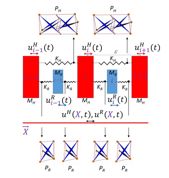
A recent study has presented a Maxwell mass–spring model for a chain formed by two different types of tensegrity prisms alternating with lumped masses. Such a model shows tensegrity theta prisms arranged in parallel with minimal regular prisms acting as resonant substructures. It features a tunable frequency bandgap response, due to the possibility of adjusting the width of the bandgap regions by playing with internal resonance effects in addition to mass and spring contrasts. This paper expands such research by presenting a continuum modeling of the tensegrity Maxwell chain, which is useful to conduct analytic studies and to develop finite element models of the plane wave dynamics of the investigated system. In correspondence to the high wave-length limit, i.e., in the low wave number regime, it is shown that the dispersion relations of the discrete and continuum models provide similar results. Analytic solutions to the wave dynamics of physical systems are presented, which validate the predictions of the bandgap response offered by the dispersion relation of the continuum model.

| [1] |
M. Kadic, G. W. Milton, M. van Hecke, M. Wegener, 3D metamaterials, Nat. Rev. Phys., 1 (2019), 198–210. https://doi.org/10.1038/s42254-018-0018-y doi: 10.1038/s42254-018-0018-y

|
| [2] |
Y. Pennec, J. O. Vasseur, B. Djafari-Rouhani, L. Dobrzyński, P. A. Deymier, Two-dimensional phononic crystals: Examples and applications, Surf. Sci. Rep., 65 (2010), 229–291. https://doi.org/10.1016/j.surfrep.2010.08.002 doi: 10.1016/j.surfrep.2010.08.002
|
| [3] |
M. Mazzotti, I. Bartoli, M. Miniaci, Modeling Bloch waves in prestressed phononic crystal plates, Front Mater, 6 (2019), 74. https://doi.org/10.3389/fmats.2019.00074 doi: 10.3389/fmats.2019.00074
|
| [4] |
A. Bergamini, M. Miniaci, T. Delpero, D. Tallarico, B. Van Damme, G. Hannema, et al., Tacticity in chiral phononic crystals, Nat Commun, 10 (2019), 4525. https://doi.org/10.1038/s41467-019-12587-7 doi: 10.1038/s41467-019-12587-7
|
| [5] |
A. S. Gliozzi, M. Miniaci, A. Chiappone, A. Bergamini, B. Morin, E. Descrovi, Tunable photo-responsive elastic metamaterials, Nat Commun, 11 (2020), 2576. https://doi.org/10.1038/s41467-020-16272-y doi: 10.1038/s41467-020-16272-y
|
| [6] |
L. Placidi, J. de Castro Motta, F. Fraternali, Bandgap structure of tensegrity mass-spring chains equipped with internal resonators, Mech. Res. Commun., 137 (2024), 104273. https://doi.org/10.1016/j.mechrescom.2024.104273 doi: 10.1016/j.mechrescom.2024.104273
|
| [7] |
E. Barchiesi, S. Khakalo, Variational asymptotic homogenization of beam-like square lattice structures, Math Mech Solids, 24 (2019), 3295–3318. https://doi.org/10.1177/1081286519843155 doi: 10.1177/1081286519843155
|
| [8] |
E. Turco, A. Misra, M. Pawlikowski, F. dell'Isola, F. Hild, Enhanced Piola–Hencky discrete models for pantographic sheets with pivots without deformation energy: numerics and experiments, Int. J. Solids. Struct., 147 (2018), 94–109. https://doi.org/10.1016/j.ijsolstr.2018.05.015 doi: 10.1016/j.ijsolstr.2018.05.015
|
| [9] |
E. Barchiesi, S. R. Eugster, L. Placidi, F. dell'Isola, Pantographic beam: a complete second gradient 1D-continuum in plane, Z. Angew. Math. Phys., 70 (2019), 1–24. https://doi.org/10.1007/s00033-018-1046-2 doi: 10.1007/s00033-018-1046-2
|
| [10] |
E. Turco, E. Barchiesi, I. Giorgio, F. dell'Isola, A Lagrangian Hencky-type non-linear model suitable for metamaterials design of shearable and extensible slender deformable bodies alternative to Timoshenko theory, Int. J. Non. Linear. Mech., 123 (2020), 103481. https://doi.org/10.1016/j.ijnonlinmec.2020.103481 doi: 10.1016/j.ijnonlinmec.2020.103481
|
| [11] | F. dell'Isola, L. Rosa, C. Wozniak, Dynamics of solids with microperiodic nonconnected fluid inclusions, Arch. Appl. Mech., (1997), 215–228. |
| [12] |
F. Fabbrocino, G. Carpentieri, A. Amendola, R. Penna, F. Fraternali, Accurate numerical methods for studying the nonlinear wave-dynamics of tensegrity metamaterials, Eccomas Procedia Compdyn, (2017), 3911–3922. https://doi.org/10.7712/120117.5693.17765 doi: 10.7712/120117.5693.17765
|
| [13] |
F. Fabbrocino, G. Carpentieri, Three-dimensional modeling of the wave dynamics of tensegrity lattices, Compos. Struct., 173 (2017), 9–16. https://doi.org/10.1016/j.compstruct.2017.03.102 doi: 10.1016/j.compstruct.2017.03.102
|
| [14] |
I. Mascolo, A. Amendola, G. Zuccaro, L. Feo, F. Fraternali, On the geometrically nonlinear elastic response of class $\theta = 1$ tensegrity prisms, Front Mater, 5 (2018), 16. https://doi.org/10.3389/fmats.2018.00016 doi: 10.3389/fmats.2018.00016
|
| [15] |
F. dell'Isola, S. R. Eugster, R. Fedele, P. Seppecher, Second-gradient continua: From Lagrangian to Eulerian and back, Math. Mech. Solids., 27 (2022), 2715–2750. https://doi.org/10.1177/10812865221078822 doi: 10.1177/10812865221078822
|
| [16] | R. E. Skelton, M. C. de Oliveira, Tensegrity Systems, New York: Springer, 2010. |
| [17] | L. D. Landau, E. M. Lifshitz, Mechanics, Third Edition: Volume 1 (Course of Theoretical Physics), Oxford: Butterworth-Heinemann, 1976. |
| [18] |
S. J. Mitchell, A. Pandolfi, M. Ortiz, Investigation of elastic wave transmission in a metaconcrete slab, Mech. Mater., 91 (2015), 295–303. https://doi.org/10.1016/j.mechmat.2015.08.004 doi: 10.1016/j.mechmat.2015.08.004
|
| [19] |
L. Placidi, F. Di Girolamo, R. Fedele, Variational study of a Maxwell–Rayleigh-type finite length model for the preliminary design of a tensegrity chain with a tunable band gap, Mech. Res. Commun., 136 (2024), 104255. https://doi.org/10.1016/j.mechrescom.2024.104255 doi: 10.1016/j.mechrescom.2024.104255
|
| [20] | F. Beer, E. Johnston, J. DeWolf, Mechanics of Materials, 5th Eds, New York: McGraw-Hill, 1999. |
| [21] |
R. Luciano, H. Darban, C. Bartolomeo, F. Fabbrocino, D. Scorza, Free flexural vibrations of nanobeams with non-classical boundary conditions using stress-driven nonlocal model, Mech. Res. Commun., 107 (2020), 103536. https://doi.org/10.1016/j.mechrescom.2020.103536 doi: 10.1016/j.mechrescom.2020.103536
|
| [22] |
H. Darban, R. Luciano, A. Caporale, F. Fabbrocino, Higher modes of buckling in shear deformable nanobeams, Int. J. Eng. Sci., 154 (2020), 103338. https://doi.org/10.1016/j.ijengsci.2020.103338 doi: 10.1016/j.ijengsci.2020.103338
|
| [23] |
A. Amendola, A. Krushynska, C. Daraio, N. M. Pugno, F. Fraternali, Tuning frequency band gaps of tensegrity metamaterials with local and global prestress, Int. J. Solids. Struct., 155 (2018), 47–56. https://doi.org/10.1016/j.ijsolstr.2018.07.002 doi: 10.1016/j.ijsolstr.2018.07.002
|
| [24] |
F. Fraternali, J. de Castro Motta, Mechanics of superelastic tensegrity braces for timber frames equipped with buckling-restrained devices, Int. J. Solids. Struct., 281 (2023), 112414. https://doi.org/10.1016/j.ijsolstr.2023.112414 doi: 10.1016/j.ijsolstr.2023.112414
|
| [25] |
F. Cornacchia, F. Fabbrocino, N. Fantuzzi, R. Luciano, R. Penna, Analytical solution of cross-and angle-ply nano plates with strain gradient theory for linear vibrations and buckling, Mech. Adv. Mater. Struct., 28 (2021), 1201–1215. https://doi.org/10.1093/isle/isab051 doi: 10.1093/isle/isab051
|
| [26] |
G. Mancusi, F. Fabbrocino, L. Feo, F. Fraternali, Size effect and dynamic properties of 2D lattice materials, Compos. B. Eng., 112 (2017), 235–242. https://doi.org/10.1016/j.compositesb.2016.12.026 doi: 10.1016/j.compositesb.2016.12.026
|
| [27] |
A. Amendola, J. de Castro Motta, G. Saccomandi, L. Vergori, A constitutive model for transversely isotropic dispersive materials, P Roy Soc A-math Phy, 480 (2024), 20230374. https://doi.org/10.1098/rspa.2023.0374 doi: 10.1098/rspa.2023.0374
|
| [28] |
J. de Castro Motta, V. Zampoli, S. Chiriţă, M. Ciarletta, On the structural stability for a model of mixture of porous solids, Math. Methods Appl. Sci., 47 (2024), 4513–4529. https://doi.org/10.1002/mma.9825 doi: 10.1002/mma.9825
|
| [29] |
K. Li, P. Rizzo, Energy harvesting using arrays of granular chains and solid rods, J. Appl. Phys., 117 (2015), 215101. https://doi.org/10.1063/1.4921856 doi: 10.1063/1.4921856
|
| [30] |
R. Misra, H. Jalali, S. J. Dickerson, P. Rizzo, Wireless module for nondestructive testing/structural health monitoring applications based on solitary waves, Sensors, 20 (2020), 3016. https://doi.org/10.3390/s20113016 doi: 10.3390/s20113016
|

Figures(2)
Luca Placidi, Julia de Castro Motta, Rana Nazifi Charandabi, Fernando Fraternali. A continuum model for the tensegrity Maxwell chain[J]. Networks and Heterogeneous Media, 2024, 19(2): 597-610. doi: 10.3934/nhm.2024026


 DownLoad: