Two-dimensional double horizon peridynamics for membranes

Zhenghao Yang; Erkan Oterkus; Selda Oterkus; Zhenghao Yang; Erkan Oterkus; Selda Oterkus

doi:10.3934/nhm.2024027

Networks and Heterogeneous Media

2024, Volume 19, Issue 2: 611-633. doi: 10.3934/nhm.2024027

Previous Article Next Article

Research article Special Issues

Two-dimensional double horizon peridynamics for membranes

1.
Otto von Guericke University, Universitätspl. 2, Magdeburg 39106, Germany
2.
PeriDynamics Research Centre, Department of Naval Architecture, Ocean and Marine Engineering, University of Strathclyde, 100 Montrose Street, Glasgow G4 0LZ, United Kingdom

Received: 24 April 2024 Revised: 10 June 2024 Accepted: 19 June 2024 Published: 21 June 2024

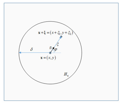
In this study, a two-dimensional "double-horizon peridynamics" formulation was presented for membranes. According to double-horizon peridynamics, each material point has two horizons: inner and outer horizons. This new formulation can reduce the computational time by using larger horizons and smaller inner horizons. To demonstrate the capability of the proposed formulation, various different analytical and numerical solutions were presented for a rectangular plate under different boundary conditions for static and dynamic problems. A comparison of peridynamic and classical solutions was given for different inner and outer horizon size values.
- Peridynamics,
- double horizon,
- nonlocal,
- classical,
- membrane,
- two-dimensional
Citation: Zhenghao Yang, Erkan Oterkus, Selda Oterkus. Two-dimensional double horizon peridynamics for membranes[J]. Networks and Heterogeneous Media, 2024, 19(2): 611-633. doi: 10.3934/nhm.2024027

Related Papers:

Abstract

In this study, a two-dimensional "double-horizon peridynamics" formulation was presented for membranes. According to double-horizon peridynamics, each material point has two horizons: inner and outer horizons. This new formulation can reduce the computational time by using larger horizons and smaller inner horizons. To demonstrate the capability of the proposed formulation, various different analytical and numerical solutions were presented for a rectangular plate under different boundary conditions for static and dynamic problems. A comparison of peridynamic and classical solutions was given for different inner and outer horizon size values.

References

[1]	S. A. Silling, Reformulation of elasticity theory for discontinuities and long-range forces, J Mech Phys Solids, 48 (2000), 175–209. https://doi.org/10.1016/S0022-5096(99)00029-0 doi: 10.1016/S0022-5096(99)00029-0
[2]	D. De Meo, L. Russo, E. Oterkus, Modeling of the onset, propagation, and interaction of multiple cracks generated from corrosion pits by using peridynamics, J Eng Mater Techn, 139 (2017), 041001. https://doi.org/10.1115/1.4036443 doi: 10.1115/1.4036443
[3]	B. B. Yin, W. K. Sun, Y. Zhang, K. M. Liew, Modeling via peridynamics for large deformation and progressive fracture of hyperelastic materials, Comput. Methods Appl. Mech. Eng., 403 (2023), 115739. https://doi.org/10.1016/j.cma.2022.115739 doi: 10.1016/j.cma.2022.115739
[4]	X. Liu, X. He, J. Wang, L. Sun, E. Oterkus, An ordinary state-based peridynamic model for the fracture of zigzag graphene sheets, Proc. Math. Phys. Eng. Sci., 474 (2018), 20180019. https://doi.org/10.1098/rspa.2018.0019 doi: 10.1098/rspa.2018.0019
[5]	M. Dorduncu, Stress analysis of sandwich plates with functionally graded cores using peridynamic differential operator and refined zigzag theory, Thin Wall Struct, 146 (2020), 106468. https://doi.org/10.1016/j.tws.2019.106468 doi: 10.1016/j.tws.2019.106468
[6]	A. Kutlu, M. Dorduncu, T. Rabczuk, A novel mixed finite element formulation based on the refined zigzag theory for the stress analysis of laminated composite plates, Compos Struct, 267 (2021), 113886. https://doi.org/10.1016/j.compstruct.2021.113886 doi: 10.1016/j.compstruct.2021.113886
[7]	W. Chen, X. Gu, Q. Zhang, X. Xia, A refined thermo-mechanical fully coupled peridynamics with application to concrete cracking, Eng. Fract. Mech., 242 (2021), 107463. https://doi.org/10.1016/j.engfracmech.2020.107463 doi: 10.1016/j.engfracmech.2020.107463
[8]	M. Qin, D. Yang, W. Chen, S. Yang, Hydraulic fracturing model of a layered rock mass based on peridynamics, Eng. Fract. Mech., 258 (2021), 108088. https://doi.org/10.1016/j.engfracmech.2021.108088 doi: 10.1016/j.engfracmech.2021.108088
[9]	A. Lakshmanan, J. Luo, I. Javaheri, V. Sundararaghavan, Three-dimensional crystal plasticity simulations using peridynamics theory and experimental comparison, Int J Plasticity, 142 (2021), 102991. https://doi.org/10.1016/j.ijplas.2021.102991 doi: 10.1016/j.ijplas.2021.102991
[10]	H. Yan, M. Sedighi, A. P. Jivkov, Peridynamics modelling of coupled water flow and chemical transport in unsaturated porous media, J Hydrol, 591 (2020), 125648. https://doi.org/10.1016/j.jhydrol.2020.125648 doi: 10.1016/j.jhydrol.2020.125648
[11]	H. Wang, S. Tanaka, S. Oterkus, E. Oterkus, Study on two-dimensional mixed-mode fatigue crack growth employing ordinary state-based peridynamics, Theor. Appl. Fract. Mech., 124 (2023), 103761. https://doi.org/10.1016/j.tafmec.2023.103761 doi: 10.1016/j.tafmec.2023.103761
[12]	Z. Yang, S. Oterkus, E. Oterkus, Peridynamic formulation for Timoshenko beam, Procedia Struct. Integr, 28 (2020), 464–471. https://doi.org/10.1016/j.prostr.2020.10.055 doi: 10.1016/j.prostr.2020.10.055
[13]	Z. Yang, E. Oterkus, S. Oterkus, Peridynamic higher-order beam formulation, J Peridyn Nonlocal Model, 3 (2021), 67–83. https://doi.org/10.1007/s42102-020-00043-w doi: 10.1007/s42102-020-00043-w
[14]	Z. Yang, B. Vazic, C. Diyaroglu, E. Oterkus, S. Oterkus, A Kirchhoff plate formulation in a state-based peridynamic framework, Math Mech Solids, 25 (2020), 727–738. https://doi.org/10.1177/1081286519887523 doi: 10.1177/1081286519887523
[15]	Z. Yang, E. Oterkus, S. Oterkus, Peridynamic formulation for higher-order plate theory, J Peridyn Nonlocal Model, 3 (2021), 185–210. https://doi.org/10.1007/s42102–020–00047–6 doi: 10.1007/s42102–020–00047–6
[16]	J. Heo, Z. Yang, W. Xia, S. Oterkus, E. Oterkus, Free vibration analysis of cracked plates using peridynamics, Ships Offshore Struct, 15 (2020), S220–S229. https://doi.org/10.1080/17445302.2020.1834266 doi: 10.1080/17445302.2020.1834266
[17]	J. Heo, Z. Yang, W. Xia, S. Oterkus, E. Oterkus, Buckling analysis of cracked plates using peridynamics, Ocean Eng., 214 (2020), 107817. https://doi.org/10.1016/j.oceaneng.2020.107817 doi: 10.1016/j.oceaneng.2020.107817
[18]	Z. Yang, C. C. Ma, E. Oterkus, S. Oterkus, K. Naumenko, Analytical solution of 1–dimensional peridynamic equation of motion, J Peridyn Nonlocal Model, 5 (2023), 356–374. https://doi.org/10.1007/s42102–022–00086–1 doi: 10.1007/s42102–022–00086–1
[19]	Z. Yang, C. C. Ma, E. Oterkus, S. Oterkus, K. Naumenko, B. Vazic, Analytical solution of the peridynamic equation of motion for a 2–dimensional rectangular membrane, J Peridyn Nonlocal Model, 5 (2023), 375–391. https://doi.org/10.1007/s42102–022–00090–5 doi: 10.1007/s42102–022–00090–5
[20]	E. Oterkus, E. Madenci, M. Nemeth, Stress analysis of composite cylindrical shells with an elliptical cutout, J mech mater struct, 2 (2007), 695–727.
[21]	T. Ni, M. Zaccariotto, Q. Z. Zhu, U. Galvanetto, Coupling of FEM and ordinary state–based peridynamics for brittle failure analysis in 3D, Mech Adv Mater Struc, 28 (2021), 875–890. https://doi.org/10.1080/15376494.2019.1602237 doi: 10.1080/15376494.2019.1602237
[22]	A. Pagani, E. Carrera, Coupling three‐dimensional peridynamics and high‐order one‐dimensional finite elements based on local elasticity for the linear static analysis of solid beams and thin‐walled reinforced structures, Int J Numer Meth Eng, 121 (2020), 5066–5081. https://doi.org/10.1002/nme.6510 doi: 10.1002/nme.6510
[23]	Y. Xia, X. Meng, G. Shen, G. Zheng, P. Hu, Isogeometric analysis of cracks with peridynamics, Comput Method Appl M, 377 (2021), 113700. https://doi.org/10.1016/j.cma.2021.113700 doi: 10.1016/j.cma.2021.113700
[24]	R. Liu, J. Yan, S. Li, Modeling and simulation of ice–water interactions by coupling peridynamics with updated Lagrangian particle hydrodynamics, Comput. Part. Mech., 7 (2020), 241–255. https://doi.org/10.1007/s40571–019–00268–7 doi: 10.1007/s40571–019–00268–7
[25]	Y. Wang, X. Zhou, Y. Wang, Y. Shou, A 3–D conjugated bond–pair–based peridynamic formulation for initiation and propagation of cracks in brittle solids, International Journal of Solids and Structures, 134 (2018), 89–115. https://doi.org/10.1016/j.ijsolstr.2017.10.022 doi: 10.1016/j.ijsolstr.2017.10.022
[26]	V. Diana, A. Bacigalupo, M. Lepidi, L. Gambarotta, Anisotropic peridynamics for homogenized microstructured materials, Comput Method Appl M, 392 (2022), 114704. https://doi.org/10.1016/j.cma.2022.114704 doi: 10.1016/j.cma.2022.114704
[27]	Y. Mikata, Peridynamics for fluid mechanics and acoustics, Acta Mech, 232 (2021), 3011–3032. https://doi.org/10.1007/s00707–021–02947–0 doi: 10.1007/s00707–021–02947–0
[28]	E. Madenci, A. Barut, M. Dorduncu, Peridynamic differential operator for numerical analysis, Berlin: Springer International Publishing, 2019,978–980. https://doi.org/10.1007/978–3–030–02647–9
[29]	H. Ren, X. Zhuang, T. Rabczuk, A higher order nonlocal operator method for solving partial differential equations, Comput Method Appl M, 367 (2020), 113132. https://doi.org/10.1016/j.cma.2020.113132 doi: 10.1016/j.cma.2020.113132
[30]	H. Ren, X. Zhuang, T. Rabczuk, A nonlocal operator method for solving partial differential equations, Comput Method Appl M, 358 (2020), 112621. https://doi.org/10.1016/j.cma.2019.112621 doi: 10.1016/j.cma.2019.112621
[31]	X. Zhuang, H. Ren, T. Rabczuk, Nonlocal operator method for dynamic brittle fracture based on an explicit phase field model, Eur J Mech A-solid, 90 (2021), 104380. https://doi.org/10.1016/j.euromechsol.2021.104380 doi: 10.1016/j.euromechsol.2021.104380
[32]	Z. Yang, E. Oterkus, S. Oterkus, C. C. Ma, Double horizon peridynamics, Math Mech Solids, 28 (2023), 2531–2549. https://doi.org/10.1177/10812865231173686 doi: 10.1177/10812865231173686
[33]	H. Ren, X. Zhuang, Y. Cai, T. Rabczuk, Dual‐horizon peridynamics, International Journal for Numerical Methods in Engineering, 108 (2016), 1451–1476. https://doi.org/10.1016/j.cma.2016.12.031 doi: 10.1016/j.cma.2016.12.031
[34]	B. Wang, S. Oterkus, E. Oterkus, Derivation of dual-horizon state-based peridynamics formulation based on Euler-Lagrange equation, Continuum Mech Therm, 35 (2023), 841–861. https://doi.org/10.1007/s00161–020–00915–y doi: 10.1007/s00161–020–00915–y
[35]	A. Javili, R. Morasata, E. Oterkus, S. Oterkus, Peridynamics review, Math Mech Solids, 24 (2019), 3714–3739. https://doi.org/10.1177/1081286518803411 doi: 10.1177/1081286518803411
[36]	E. Madenci, E. Oterkus, Peridynamic Theory and Its Applications, New York: Springer New York, 2013. https://doi.org/10.1007/978–1–4614–8465–3
[37]	L. Lopez, S. F. Pellegrino, A space-time discretization of a nonlinear peridynamic model on a 2D lamina, Comput Math Appl, 116 (2022), 161–175. https://doi.org/10.1016/j.camwa.2021.07.004 doi: 10.1016/j.camwa.2021.07.004
[38]	S. Jafarzadeh, A. Larios, F. Bobaru, Efficient solutions for nonlocal diffusion problems via boundary-adapted spectral methods, J Peridyn Nonlocal Model, 2 (2020), 85–110. https://doi.org/10.1007/s42102–019–00026–6 doi: 10.1007/s42102–019–00026–6

Reader Comments

Your name:*

Email:*
© 2024 the Author(s), licensee AIMS Press. This is an open access article distributed under the terms of the Creative Commons Attribution License (http://creativecommons.org/licenses/by/4.0)