Alkaptonuria (AKU) is a rare metabolic disease which is inherited as an autosomal recessive trait. It is characterized by the accumulation of homogentisic acid over time in various tissues of the body particularly connective tissues. This genetic disease is caused by mutation of the Homogentisate 1,2-dioxygenase (HGD) gene which encodes for enzyme essential for the catabolism of phenylalanine and tyrosine. The aim of the present study is to investigate variant types in Jordanian patients with alkaptonuria. Genomic DNA was extracted from whole blood samples of the participated AKU family members (n = 23). The 14 exons of HGD gene for the proband were amplified using specific PCR primers. The sequenced data were analysed and the pathogenicity of the identified variants were predicted using the online bioinformatics programs: PolyPhen2, SIFT and Mutation taster. The analysis showed that the proband was compound heterozygous for the missense mutations A122V and R225C found within E6 and E10, respectively. R225C variant is novel and the genotyping of the family members indicated that HGDA122V and HGDR225C alleles were fully segregated. Moreover, the cousins of the proband who are AKU patients inherited the homozygous pattern of the novel mutation. This study extends the pathogenic mutations spectrum of the HGD gene. It identified the novel mutation R225C and at the same time confirmed the high prevalence of the founder mutation A122V in Jordanian AKU patients.
Citation: Nesrin R. Mwafi, Dema A. Ali, Raida W. Khalil, Ibrahim N. Alsbou', Ahmad M. Saraireh. Novel R225C variant identified in the HGD gene in Jordanian patients with alkaptonuria[J]. AIMS Molecular Science, 2021, 8(1): 60-75. doi: 10.3934/molsci.2021005
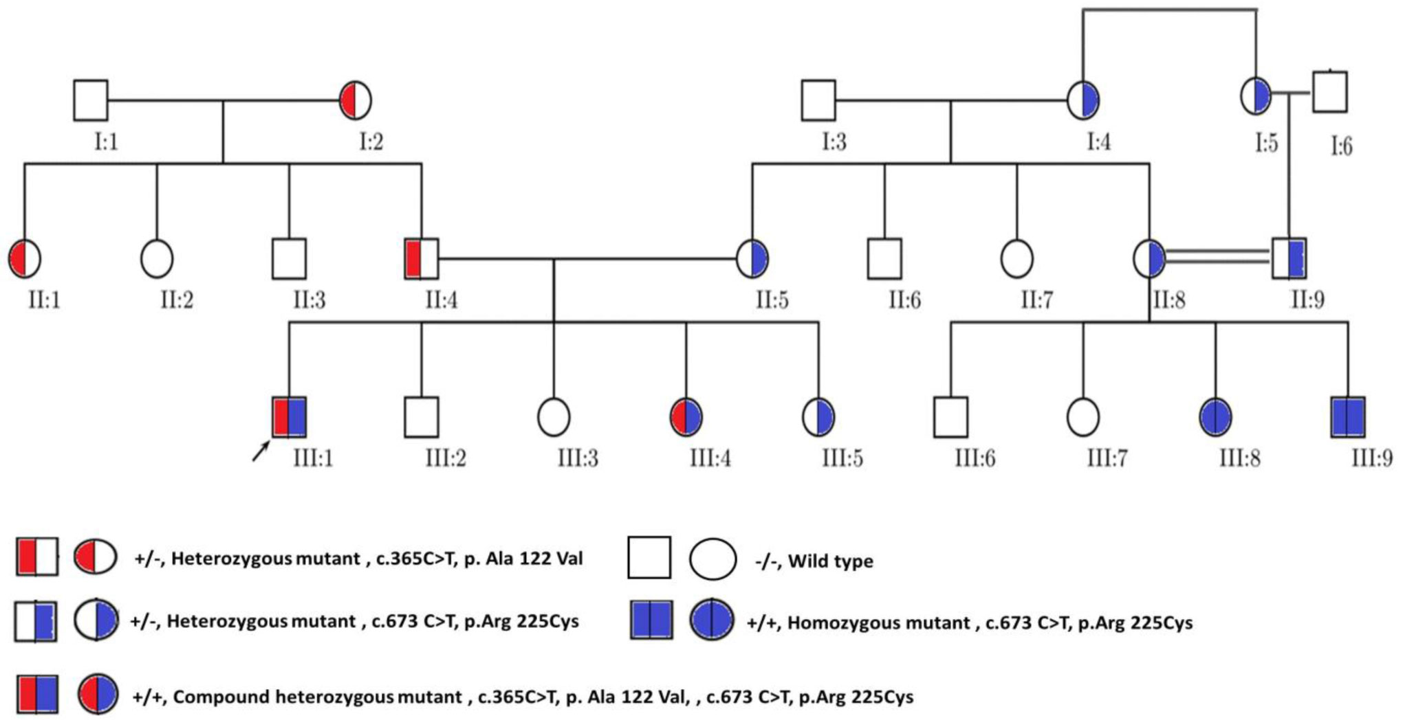
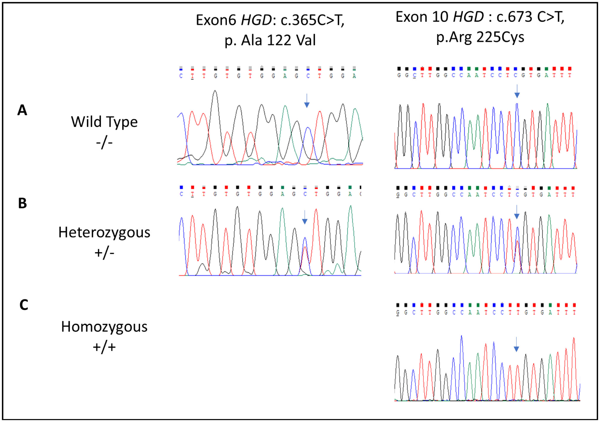
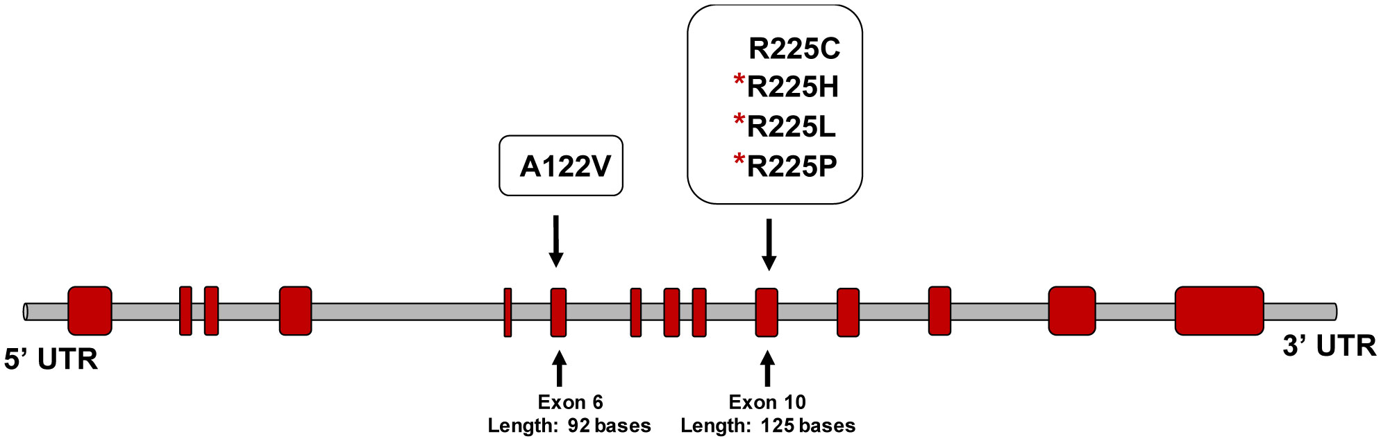
Alkaptonuria (AKU) is a rare metabolic disease which is inherited as an autosomal recessive trait. It is characterized by the accumulation of homogentisic acid over time in various tissues of the body particularly connective tissues. This genetic disease is caused by mutation of the Homogentisate 1,2-dioxygenase (HGD) gene which encodes for enzyme essential for the catabolism of phenylalanine and tyrosine. The aim of the present study is to investigate variant types in Jordanian patients with alkaptonuria. Genomic DNA was extracted from whole blood samples of the participated AKU family members (n = 23). The 14 exons of HGD gene for the proband were amplified using specific PCR primers. The sequenced data were analysed and the pathogenicity of the identified variants were predicted using the online bioinformatics programs: PolyPhen2, SIFT and Mutation taster. The analysis showed that the proband was compound heterozygous for the missense mutations A122V and R225C found within E6 and E10, respectively. R225C variant is novel and the genotyping of the family members indicated that HGDA122V and HGDR225C alleles were fully segregated. Moreover, the cousins of the proband who are AKU patients inherited the homozygous pattern of the novel mutation. This study extends the pathogenic mutations spectrum of the HGD gene. It identified the novel mutation R225C and at the same time confirmed the high prevalence of the founder mutation A122V in Jordanian AKU patients.
Alkaptonuria
Gas Chromatography-Mass Spectrometry analysis
multiplex ligation-dependent probe amplification

| [1] |
Garrod AE (1902) The Incidence of Alkaptonuria: A Study in Chemical Individuality. Lancet 2: 1616-1620. doi: 10.1016/S0140-6736(01)41972-6

|
| [2] | Garrod AE (1908) The Croonian Lectures on inborn errors of metabolism, lecture II Alkaptonuria. Lancet 2: 73-79. |
| [3] |
Phornphutkul C, Introne WJ, Perry MB, et al. (2002) Natural history of alkaptonuria. N Engl J Med 347: 2111-2121. doi: 10.1056/NEJMoa021736
|
| [4] | Mistry JB, Bukhari M, Taylor AM (2013) Alkaptonuria. Rare Dis 1: 1-7. |
| [5] |
La Du BN, Zannoni VG, Laster L, et al. (1958) The nature of the defect in tyrosine metabolism in alcaptonuria. J Biol Chem 230: 251-260. doi: 10.1016/S0021-9258(18)70560-7
|
| [6] |
Al-Shagahin HM, Mwafi N, Khasawneh M, et al. (2019) Ear, nose, and throat manifestations of alkaptonuria patients from Jordan. Indian J Otol 25: 109-113. doi: 10.4103/indianjotol.INDIANJOTOL_23_19
|
| [7] |
Sakthivel S, Zatkova A, Nemethova M, et al. (2014) Mutation screening of the HGD gene identifies a novel alkaptonuria mutation with significant founder effect and high prevalence. Ann Hum Genet 78: 155-164. doi: 10.1111/ahg.12055
|
| [8] | Helliwell TR, Gallagher JA, Ranganath L (2008) Alkaptonuria--a review of surgical and autopsy pathology. Histopathology 53: 503-512. |
| [9] |
Fernandez-Canon JM, Granadino B, Beltran-Valero de Bernabe D, et al. (1996) The molecular basis of alkaptonuria. Nat Genet 14: 19-24. doi: 10.1038/ng0996-19
|
| [10] |
Zatkova A (2011) An update on molecular genetics of Alkaptonuria (AKU). J Inherit Metab Dis 34: 1127-1136. doi: 10.1007/s10545-011-9363-z
|
| [11] |
Alsbou M, Mwafi N (2013) A previously undiagnosed case of alkaptonuria: A case report. Turk J Rheumatol 28: 132-135. doi: 10.5606/tjr.2013.2660
|
| [12] | Ranganath LR, Milan AM, Hughes AT, et al. (2020) Reversal of ochronotic pigmentation in alkaptonuria following nitisinone therapy: Analysis of data from the United Kingdom National Alkaptonuria Centre. JIMD Rep 1-13. |
| [13] |
Zatkova A, Ranganath L, Kadasi L (2020) Alkaptonuria: Current Perspectives. Appl Clin Genet 13: 37-47. doi: 10.2147/TACG.S186773
|
| [14] |
Ranganath LR, Jarvis JC, Gallagher JA (2013) Recent advances in management of alkaptonuria (invited review; best practice article). J Clin Pathol 66: 367-373. doi: 10.1136/jclinpath-2012-200877
|
| [15] |
Taylor AM, Boyde A, Wilson PJ, et al. (2011) The role of calcified cartilage and subchondral bone in the initiation and progression of ochronotic arthropathy in alkaptonuria. Arthritis Rheum 63: 3887-3896. doi: 10.1002/art.30606
|
| [16] | Wu K, Bauer E, Myung G, et al. (2018) Musculoskeletal manifestations of alkaptonuria: A case report and literature review. Eur J Rheumatol 6: 98-101. |
| [17] |
Thapa M, Yu J, Lee W, et al. (2015) Determination of homogentisic acid in human plasma by GC-MS for diagnosis of alkaptonuria. Anal Sci Technol 28: 323-330. doi: 10.5806/AST.2015.28.5.323
|
| [18] | Groseanu L, Marinescu R, Laptoiun D, et al. (2010) A late and difficult diagnosis of ochronosis. J Med Life 3: 437-443. |
| [19] |
Balaban B, Taskaynatan M, Yasar E, et al. (2006) Ochronotic spondyloarthropathy: Spinal involvement resembling ankylosing spondylitis. Clin Rheumatol 25: 598-601. doi: 10.1007/s10067-005-0038-8
|
| [20] |
Ranganath LR, Milan AM, Hughes AT, et al. (2016) Suitability Of Nitisinone In Alkaptonuria 1 (SONIA 1): an international, multicentre, randomised, open-label, no-treatment controlled, parallel-group, dose-response study to investigate the effect of once daily nitisinone on 24-h urinary homogentisic acid excretion in patients with alkaptonuria after 4 weeks of treatment. Ann Rheum Dis 75: 362-367. doi: 10.1136/annrheumdis-2014-206033
|
| [21] |
Ranganath LR, Psarelli EE, Arnoux J, et al. (2020) Efficacy and safety of once-daily nitisinone for patients with alkaptonuria (SONIA 2): an international, multicentre, open-label, randomised controlled trial. Lancet Diabetes Endocrinol 8: 762-772. doi: 10.1016/S2213-8587(20)30228-X
|
| [22] |
Ranganath LR, Khedr M, Milan AM, et al. (2018) Nitisinone arrests ochronosis and decreases rate of progression of Alkaptonuria: Evaluation of the effect of nitisinone in the United Kingdom National Alkaptonuria Centre. Mol Genet Metab 125: 127-134. doi: 10.1016/j.ymgme.2018.07.011
|
| [23] |
Keenan CM, Preston AJ, Sutherland H, et al. (2015) Nitisinone Arrests but Does Not Reverse Ochronosis in Alkaptonuric Mice. JIMD Rep 24: 45-50. doi: 10.1007/8904_2015_437
|
| [24] |
Khedr M, Judd S, Briggs MC, et al. (2018) Asymptomatic Corneal Keratopathy Secondary to Hypertyrosinaemia Following Low Dose Nitisinone and a Literature Review of Tyrosine Keratopathy in Alkaptonuria. JIMD Rep 40: 31-37. doi: 10.1007/8904_2017_62
|
| [25] |
Hughes JH, Wilson P, Sutherland H, et al. (2020) Dietary restriction of tyrosine and phenylalanine lowers tyrosinemia associated with nitisinone therapy of alkaptonuria. J Inherit Metab Dis 43: 259-268. doi: 10.1002/jimd.12172
|
| [26] |
Kılavuz S, Derya Bulut F, Kör D, et al. (2018) Demographic, Phenotypic and Genotypic Features of Alkaptonuria Patients: A Single Centre Experience. J Pediatr Res 3: 7-11. doi: 10.4274/jpr.20982
|
| [27] |
Ascher DB, Spiga O, Sekelska M, et al. (2019) Homogentisate 1,2-dioxygenase (HGD) gene variants, their analysis and genotype–phenotype correlations in the largest cohort of patients with AKU. Eur J Hum Genet 27: 888-902. doi: 10.1038/s41431-019-0354-0
|
| [28] |
Zatkova A, Sedlackova T, Radvansky J, et al. (2012) Identification of 11 Novel Homogentisate 1, 2 Dioxygenase Variants in Alkaptonuria Patients and Establishment of a Novel LOVD-Based HGD Mutation Database. JIMD Rep 4: 55-65. doi: 10.1007/8904_2011_68
|
| [29] |
Abdulrazzaq YM, Ibrahim A, Al-khayat AI, et al. (2009) R58fs mutation in the HGD gene in a family with alkaptonuria in the UAE. Ann Hum Genet 73: 125-130. doi: 10.1111/j.1469-1809.2008.00485.x
|
| [30] |
Ladjouze-Rezig A, Rodriguez de Cordoba S, Aquaron R (2006) Ochronotic rheumatism in Algeria: clinical, radiological, biological and molecular studies- a case study of 14 patients in 11 families. Joint Bone Spine 73: 284-292. doi: 10.1016/j.jbspin.2005.03.010
|
| [31] |
Al-Sbou M, Mwafi N, Lubad MA (2012) Identification of forty cases with alkaptonuria in one village in Jordan. Rheumatol Int 32: 3737-3740. doi: 10.1007/s00296-011-2219-x
|
| [32] |
Nemethova M, Radvanszky J, Kadasi L, et al. (2016) Twelve novel HGD gene variants identified in 99 alkaptonuria patients: Focus on “black bone disease” in Italy. Eur J Hum Genet 24: 66-72. doi: 10.1038/ejhg.2015.60
|
| [33] |
Koressaar T, Remm M (2007) Enhancements and modifications of primer design program Primer3. Bioinformatics 23: 1289-1291. doi: 10.1093/bioinformatics/btm091
|
| [34] |
Untergasser A, Cutcutache I, Koressaar T, et al. (2012) Primer3-new capabilities and interfaces. Nucleic Acids Res 40: e115. doi: 10.1093/nar/gks596
|
| [35] | Zatkova A, Nemethova M (2015) Genetics of alkaptonuria – an overview. Eur Pharm J 62: 27-32. |
| [36] |
Ben Halim N, Ben Alaya Bouafif N, Romdhane L, et al. (2013) Consanguinity, endogamy, and genetic disorders in Tunisia. J Community Genet 4: 273-284. doi: 10.1007/s12687-012-0128-7
|
| [37] | Hamamy HA, Masri AT, Al-Hadidy AM, et al. (2007) Consanguinity and genetic disorders. Profile from Jordan. Saudi Med J 28: 1015-1017. |
| [38] |
Titus GP, Mueller HA, Burgner J, et al. (2000) Crystal structure of human homogentisate dioxygenase. Nat Struct Biol 7: 542-546. doi: 10.1038/76756
|
| [39] |
Usher J, Ascher D, Pires D, et al. (2015) Analysis of HGD Gene Mutations in Patients with Alkaptonuria from the United Kingdom: Identification of Novel Mutations. JIMD Rep 24: 3-11. doi: 10.1007/8904_2014_380
|
| [40] |
Bernini A, Galderisi S, Spiga O, et al. (2017) Toward a generalized computational workflow for exploiting transient pockets as new targets for small molecule stabilizers: application to the homogentisate 1,2-dioxygenase mutants at the base of rare disease Alkaptonuria. Comput Biol Chem 70: 133-141. doi: 10.1016/j.compbiolchem.2017.08.008
|
| [41] |
Vilboux T, Kayser M, Introne W, et al. (2009) Mutation spectrum of homogentisic acid oxidase (HGD) in alkaptonuria. Hum Mutat 30: 1611-1619. doi: 10.1002/humu.21120
|
| [42] |
Beltrán-Valero De Bernabé D, Granadino B, Chiarelli I, et al. (1998) Mutation and polymorphism analysis of the human homogentisate 1,2-dioxygenase gene in alkaptonuria patients. Am J Hum Genet 62: 776-784. doi: 10.1086/301805
|
Figures(5) / Tables(3)

Nesrin R. Mwafi, Dema A. Ali, Raida W. Khalil, Ibrahim N. Alsbou', Ahmad M. Saraireh. Novel R225C variant identified in the HGD gene in Jordanian patients with alkaptonuria[J]. AIMS Molecular Science, 2021, 8(1): 60-75. doi: 10.3934/molsci.2021005


 DownLoad: