Climate change is an inevitable and important problem faced worldwide. Around the world, many researchers are doing research work on climate change with different factors. The authors of this study have used the fractal dimension to analyze the $ 41 $ years of climate change in India, from $ 1981 $ to $ 2021 $. The meteorological parameters, surface pressure, temperature, wind speed, and precipitation of $ 45 $ places in India were investigated for this research study. Each parameter was individually examined. As a result of this research, the mean average fractal dimension value of all parameters was acquired from $ 1.184 $ to $ 1.198 $. It was found that all the parameters within the data set, had a long-term persistence behavior. With these values, a suggestion for the prediction of the parameters was proposed. The results of the integrated analysis of these parameters showed that, with the exception of a location, all landscapes had a feature that precipitation increased with the temperature. Moreover, with the exception of two landscapes (the island and the frosty mountains), all areas received heavy rainfall during periods of low wind. Thus, this study contributes to a better understanding of the fractal aspects of climate change and the complexity of irregularity and the classification of weather characteristics.
Citation: M. Meenakshi, A. Gowrisankar, Jinde Cao, Pankajam Natarajan. Fractal dimension approach on climate analysis of India[J]. Mathematical Modelling and Control, 2025, 5(1): 15-30. doi: 10.3934/mmc.2025002
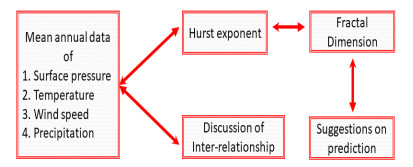
Climate change is an inevitable and important problem faced worldwide. Around the world, many researchers are doing research work on climate change with different factors. The authors of this study have used the fractal dimension to analyze the $ 41 $ years of climate change in India, from $ 1981 $ to $ 2021 $. The meteorological parameters, surface pressure, temperature, wind speed, and precipitation of $ 45 $ places in India were investigated for this research study. Each parameter was individually examined. As a result of this research, the mean average fractal dimension value of all parameters was acquired from $ 1.184 $ to $ 1.198 $. It was found that all the parameters within the data set, had a long-term persistence behavior. With these values, a suggestion for the prediction of the parameters was proposed. The results of the integrated analysis of these parameters showed that, with the exception of a location, all landscapes had a feature that precipitation increased with the temperature. Moreover, with the exception of two landscapes (the island and the frosty mountains), all areas received heavy rainfall during periods of low wind. Thus, this study contributes to a better understanding of the fractal aspects of climate change and the complexity of irregularity and the classification of weather characteristics.

| [1] |
L. Schipper, M. Pelling, Disaster risk, climate change and international development: scope for, and challenges to, integration, Disasters, 30 (2006), 19–38. https://doi.org/10.1111/j.1467-9523.2006.00304.x doi: 10.1111/j.1467-9523.2006.00304.x

|
| [2] |
A. Gowrisankar, T. M. C. Priyanka, A. Saha, L. Rondoni, K. Hassan, S. Banerjee, Greenhouse gas emissions: a rapid submerge of the world, Chaos, 6 (2022), 1–32. https://doi.org/10.1063/5.0091843 doi: 10.1063/5.0091843
|
| [3] |
E. Ostrom, Polycentric systems for coping with collective action and global environmental change, Global Just., 20 (2017), 423–430. https://doi:10.1016/j.gloenvcha.2010.07.004 doi: 10.1016/j.gloenvcha.2010.07.004
|
| [4] |
V. P. Tewari, R. K.Verma, K. Von Gadow, Climate change effects in the Western Himalayan ecosystems of India: evidence and strategies, Forest Ecosyst., 4 (2017), 1–9. https://doi.org/10.1186/s40663-017-0100-4 doi: 10.1186/s40663-017-0100-4
|
| [5] |
B. Chapman, K. Rosemond, Seasonal climate summary for the southern hemisphere (autumn 2018): a weak La Nina fades, the austral autumn remains warmer and drier, J. South. Hemisphere Earth Syst. Sci., 70 (2020), 328–352. https://doi.org/10.1071/ES19039 doi: 10.1071/ES19039
|
| [6] |
A. M. Makarieva, V. G. Gorshkov, D. Sheil, A. D. Nobre, B. L. Li, Where do winds come from? A new theory on how water vapor condensation influences atmospheric pressure and dynamics, Atmos. Chem. Phys., 13 (2013), 1039–1056. https://doi.org/10.5194/acp-13-1039-2013 doi: 10.5194/acp-13-1039-2013
|
| [7] |
J. H. Van Hateren, A fractal climate response function can simulate global average temperature trends of the modern era and the past millennium, Clim. Dyn., 40 (2013), 2651–2670. https://doi.org/10.1007/s00382-012-1375-3 doi: 10.1007/s00382-012-1375-3
|
| [8] | S. Eichelberger, J. McCaa, B. Nijssen, A. Wood, Climate change effects on wind speed, North Amer. Windpower, 7 (2008), 68–72. |
| [9] |
K. E. Trenberth, Changes in precipitation with climate change, Climate Res., 47 (2011) 123–138. https://doi.org/10.3354/cr00953 doi: 10.3354/cr00953
|
| [10] |
B. B. Mandelbrot, J. R. Wallis, Some long‐run properties of geophysical records, Water Resour. Res., 5 (1969), 321–340. https://doi.org/10.1029/WR005i002p00321 doi: 10.1029/WR005i002p00321
|
| [11] |
L. Bodri, Fractal analysis of climatic data: Mean annual temperature records in Hungary, Theor. Appl. Climatology, 49 (1994), 53–57. https://doi.org/10.1007/BF00866288 doi: 10.1007/BF00866288
|
| [12] |
R. Govindan, D. A. Sant, Fractal dimensional analysis of Indian climatic dynamics, Chaos Solitons Fract., 19 (2004), 285–291. https://doi.org/10.1016/S0960-0779(03)00042-0 doi: 10.1016/S0960-0779(03)00042-0
|
| [13] |
N. C. Sahu, D. Mishra, Analysis of perception and adaptability strategies of the farmers to climate change in Odisha, India, APCBEE Proc., 5 (2013), 123–127. https://doi.org/10.1016/j.apcbee.2013.05.022 doi: 10.1016/j.apcbee.2013.05.022
|
| [14] |
S. Rehman, A. H. Siddiqi, Wavelet based Hurst exponent and fractal dimensional analysis of Saudi climatic dynamics, Chaos Solitons Fract., 40 (2009), 1081–1090. https://doi.org/10.1016/j.chaos.2007.08.063 doi: 10.1016/j.chaos.2007.08.063
|
| [15] |
B. Cui, P. Huang, W. Xie, Fractal dimension characteristics of wind speed time series under typhoon climate, J. Wind Eng. Ind. Aerodyn., 229 (2022), 105144. https://doi.org/10.1016/j.jweia.2022.105144 doi: 10.1016/j.jweia.2022.105144
|
| [16] |
M. Li, Fractal time series–a tutorial review, Math. Probl. Eng., 2010 (2010), 157264. https://doi.org/10.1155/2010/157264 doi: 10.1155/2010/157264
|
| [17] | D. W. Stroock, Probability theory: an analytic view, Cambridge University Press, 2010. |
| [18] | J. Feder, Fractals, Springer Science & Business Media, 2013. https://doi.org/10.1007/978-1-4899-2124-6 |
| [19] | S. Banerjee, M. K. Hassan, S. Mukherjee, A. Gowrisankar, Fractal patterns in nonlinear dynamics and applications, CRC Press, 2020. |
| [20] |
H. E. Hurst, Long-term storage capacity of reservoirs, Trans. Amer. Soc. Civ. Eng., 116 (1951), 770–799. https://doi.org/10.1061/TACEAT.0006518 doi: 10.1061/TACEAT.0006518
|
| [21] | B. Qian, K. Rasheed, Hurst exponent and financial market predictability IASTED Conference on Financial Engineering and Applications, 2004,203–209. |
| [22] |
A. Akhrif, M. Romanos, K. Domschke, A. Schmitt-Boehrer, S. Neufang, Fractal analysis of BOLD time series in a network associated with waiting impulsivity, Front. Physiol., 9 (2018), 1378. https://doi.org/10.3389/fphys.2018.01378 doi: 10.3389/fphys.2018.01378
|
| [23] |
M. F. Barnsley, S. Demko, Iterated function systems and the global construction of fractals, Proc. R. Soc. London. A, 399 (1985), 243–275. https://doi.org/10.1098/rspa.1985.0057 doi: 10.1098/rspa.1985.0057
|
| [24] | M. F. Barnsley, Fractals everywhere, Academic Press, 2014. https://doi.org/10.1016/c2013-0-10335-2 |
| [25] | S. Banerjee, D. Easwaramoorthy, A. Gowrisankar, Fractal functions, dimensions and signal analysis, Springer, 2021. https://doi.org/10.1007/978-3-030-62672-3 |
| [26] |
B. B. Mandelbrot, Self-affine fractals and fractal dimension, Phys. Scr., 32 (1985), 257. https://doi.org/ 10.1088/0031-8949/32/4/001 doi: 10.1088/0031-8949/32/4/001
|
| [27] |
C. Thangaraj, D. Easwaramoorthy, Generalized fractal dimensions based comparison analysis of edge detection methods in CT images for estimating the infection of COVID-19 disease, Eur. Phys. J. Special Top., 231 (2022), 3717–3739. https://doi.org/10.1140/epjs/s11734-022-00651-1 doi: 10.1140/epjs/s11734-022-00651-1
|
| [28] | Y. Kohavi, H. Davdovich, Topological dimensions, Hausdorff dimensions & fractals, Bar-llan University, 2006. |
| [29] |
I. Pilgrim, R. P. Taylor, Fractal analysis of time-series data sets: methods and challenges, Fractal Anal., 20 (2018), 5–30. https://doi.org/10.5772/intechopen.81958 doi: 10.5772/intechopen.81958
|
| [30] |
J. B. Bassingthwaighte, G. M. Raymond, Evaluating rescaled range analysis for time series, Ann. Biomed. Eng., 22, (1994), 432–444. https://doi.org/10.1007/BF02368250 doi: 10.1007/BF02368250
|
| [31] |
S. Lovejoy, B. B. Mandelbrot, Fractal properties of rain, and a fractal model, Tellus A, 37 (1985), 209–232. https://doi.org/10.1111/j.1600-0870.1985.tb00423.x doi: 10.1111/j.1600-0870.1985.tb00423.x
|
| [32] |
H. Tatli, Detecting persistence of meteorological drought via the Hurst exponent, Meteorol. Appl., 22 (2015), 763–769. https://doi.org/10.1002/met.1519 doi: 10.1002/met.1519
|


Figures(9) / Tables(4)
M. Meenakshi, A. Gowrisankar, Jinde Cao, Pankajam Natarajan. Fractal dimension approach on climate analysis of India[J]. Mathematical Modelling and Control, 2025, 5(1): 15-30. doi: 10.3934/mmc.2025002


 DownLoad: