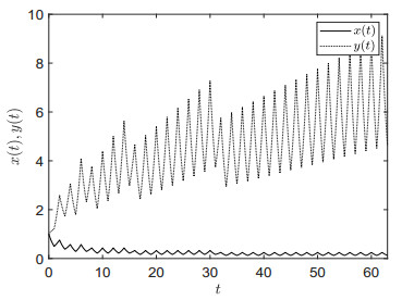
Mainly addressed in this paper is the stability problem of continuous-time switched cascade nonlinear systems with time-varying delays. A robust convergence property is proved first: If a nominal switched nonlinear system with delays is asymptotically stable, then trajectories of corresponding perturbed system asymptotically approach origin provided that the perturbation can be upper bounded by a function exponentially decaying to zero. Applying this property and assuming that a cascade system consists of two separate systems, it is shown that a switched cascade nonlinear system is asymptotically stable if one separate system is exponentially stable and the other one is asymptotically stable. Since the considered switching signals have a uniform property and thus include most switching signals frequently encountered, our results are valid for a wide range of switched cascade systems.
Citation: Xingwen Liu, Shouming Zhong. Stability analysis of delayed switched cascade nonlinear systems with uniform switching signals[J]. Mathematical Modelling and Control, 2021, 1(2): 90-101. doi: 10.3934/mmc.2021007
Mainly addressed in this paper is the stability problem of continuous-time switched cascade nonlinear systems with time-varying delays. A robust convergence property is proved first: If a nominal switched nonlinear system with delays is asymptotically stable, then trajectories of corresponding perturbed system asymptotically approach origin provided that the perturbation can be upper bounded by a function exponentially decaying to zero. Applying this property and assuming that a cascade system consists of two separate systems, it is shown that a switched cascade nonlinear system is asymptotically stable if one separate system is exponentially stable and the other one is asymptotically stable. Since the considered switching signals have a uniform property and thus include most switching signals frequently encountered, our results are valid for a wide range of switched cascade systems.

| [1] | X. Lin, W. Zhang, S. Huang, and E. Zheng, Finite-time stabilization of input-delay switched systems, Applied Mathematics & Computation, 375 (2020), 125062. |
| [2] | Y. Li, Y. Sun, F. Meng, and Y. Tian, Exponential stabilization of switched time-varying systems with delays and disturbances, Applied Mathematics & Computation, 324 (2018), 131–140. |
| [3] |
X. Liu, Q. Zhao, and S. Zhong, Stability analysis of a class of switched nonlinear systems with delays: A trajectory-based comparison method, Automatica, 91 (2018), 36–42. doi: 10.1016/j.automatica.2018.01.018

|
| [4] | A. Aleksandrov and O. Mason, Diagonal stability of a class of discrete-time positive switched systems with delay, IET Control Theory & Applications, 12 (2018), 812–818. |
| [5] | W. Ren and J. Xiong, Krasovskii and Razumikhin stability theorems for stochastic switched nonlinear time-delay systems, SIAM Journal on Control & Optimization, 57 (2019), 1043–1067. |
| [6] | W. Michiels, R. Sepulchre, and D. Roose, Stability of perturbed delay differential equations and stabilization of nonlinear cascade systems, SIAM Journal on Control & Optimization, 40 (2001), 661–680. |
| [7] | H. Hammouri and M. Sahnoun, Nonlinear observer based on cascade form and output injection, SIAM Journal on Control & Optimization, 53 (2015), 3195–3227. |
| [8] | T. Bayen, A. Rapaport, and M. Sebbah, Minimal time control of the two tanks gradostat model under a cascade input constraint, SIAM Journal on Control & Optimization, 52 (2014), 2568–2594. |
| [9] |
X. Zhang, W. Lin, and Y. Lin, Dynamic partial state feedback control of cascade systems with time-delay, Automatica, 77 (2017), 370–379. doi: 10.1016/j.automatica.2016.09.037
|
| [10] |
S. Zhao, G. M. Dimirovski, and R. Ma, Robust $H_\infty$ control for non-minimum phase switched cascade systems with time delay, Asian Journal of Control, 17 (2015), 1–10. doi: 10.1002/asjc.1056
|
| [11] | B. Niu and J. Zhao, Robust $H_\infty$ control for a class of switched nonlinear cascade systems via multiple Lyapunov functions approach, Applied Mathematics & Computation, 218 (2012), 6330–6339. |
| [12] | X. Dong, L. Chang, F. Wu, and N. Hu, Tracking control for switched cascade nonlinear systems, Mathematical Problems in Engineering, 2015 (2015), 105646. |
| [13] |
M. Wang, J. Zhao, and G. M. Dimirovski, $H_\infty$ control for a class of cascade switched nonlinear systems, Asian Journal of Control, 10 (2008), 724–729. doi: 10.1002/asjc.73
|
| [14] |
X. Liu, S. Zhong, and Q. Zhao, Dynamics of delayed switched nonlinear systems with applications to cascade systems, Automatica, 87 (2018), 251–257. doi: 10.1016/j.automatica.2017.10.012
|
| [15] | Q. Su, X. Jia, and H. Liu, Finite-time stabilization of a class of cascade nonlinear switched systems under state-dependent switching, Applied Mathematics & Computation, 289 (2016), 172–180. |
| [16] | X. Liu, Q. Zhao, Robust convergence of discrete-time delayed switched nonlinear systems and its applications to cascade systems, International Journal of Robust & Nonlinear Control, 28 (2018), 767–780. |
| [17] |
Z. Chen, Global stabilization of nonlinear cascaded systems with a Lyapunov function in superposition form, Automatica, 45 (2009), 2041–2045. doi: 10.1016/j.automatica.2009.04.021
|
| [18] | P. Forni, D. Angeli, Input-to-state stability for cascade systems with multiple invariant sets, Systems & Control Letters, 98 (2016), 97–110. |
| [19] | M. Wang, J. Zhao, G. Dimirovski, Variable structure control method to the output tracking control of cascade non-linear switched systems, IET Control Theory & Applications, 3 (2009), 1634–1640. |
| [20] | H. K. Khalil, Nonlinear Control. Paris: Pearson, 2015. |
| [21] | H. K. Khalil, Nonlinear Systems, 3rd ed. London: Prentice Hall, 2002. |
| [22] |
X. Liu, S. Zhong, Asymptotic stability analysis of discrete-time switched cascade nonlinear systems with delays, IEEE Trans. on Automatic Control, 65 (2020), 2686–2692. doi: 10.1109/TAC.2019.2942009
|
| [23] |
P. Pepe, G. Pola, M. D. Di Benedetto On Lyapunov-Krasovskii characterizations of stability notions for discrete-time systems with uncertain time-varying time-delays, IEEE Trans. on Automatic Control, 63 (2018), 1603–1617. doi: 10.1109/TAC.2017.2749526
|
| [24] | D. Liberzon, Switching in Systems and Control, Boston: Springer Verlag (2003). |
| [25] | M. Porfiri, D. G. Roberson, D. J. Stilwell, Fast switching analysis of linear switched systems using exponential splitting, SIAM Journal on Control & Optimization, 47 (2008), 2582–2597. |
| [26] | X. Zhao, P. Shi, Y. Yin, S. K. Nguang, New results on stability of slowly switched systems: A multiple discontinuous Lyapunov function approach, IEEE Trans. on Automatic Control, 62 (2013), 3502–3509. |
| [27] |
P. Bolzern, P. Colaneri, G. De Nicolao, Almost sure stability of Markov jump linear systems with deterministic switching, IEEE Trans. on Automatic Control, 58 (2013), 209–213. doi: 10.1109/TAC.2012.2203049
|
| [28] | D. Zhai, A.-Y. Lu, J.-H. Li, Q.-L. Zhang, Simultaneous fault detection and control for switched linear systems with mode-dependent average dwell-time, Applied Mathematics & Computation, 273 (2016), 767–792. |
| [29] |
A. Lamperski, A. D. Ames, Lyapunov theory for zeno stability, IEEE Trans. on Automatic Control, 58 (2013), 100–112. doi: 10.1109/TAC.2012.2208292
|
| [30] | M. S. Mahmoud, New York: Springer, Switched Time-Delay Systems: Stability and Control, 49 (2010), 305–307. |
| [31] |
Y. Li, Y. Sun, F. Meng, New criteria for exponential stability of switched time-varying systems with delays and nonlinear disturbances, Nonlinear Analysis: Hybrid Systems, 26 (2017), 284–291. doi: 10.1016/j.nahs.2017.06.007
|
| [32] |
Y. Sun, L. Wang, On stability of a class of switched nonlinear systems, Automatica, 49 (2013), 305–307. doi: 10.1016/j.automatica.2012.10.011
|


Figures(3)
Xingwen Liu, Shouming Zhong. Stability analysis of delayed switched cascade nonlinear systems with uniform switching signals[J]. Mathematical Modelling and Control, 2021, 1(2): 90-101. doi: 10.3934/mmc.2021007


 DownLoad: