Persistence and extinction of infection in stochastic population model with horizontal and imperfect vertical disease transmissions

Abhijit Majumder; Debadatta Adak; Adeline Samson; Nandadulal Bairagi; Abhijit Majumder; Debadatta Adak; Adeline Samson; Nandadulal Bairagi

doi:10.3934/mbe.2025030

Mathematical Biosciences and Engineering

2025, Volume 22, Issue 4: 846-875. doi: 10.3934/mbe.2025030

Previous Article Next Article

Research article Special Issues

Persistence and extinction of infection in stochastic population model with horizontal and imperfect vertical disease transmissions

1.
Department of Biological Sciences and Eck Institute for Global Health, University of Notre Dame, Notre Dame, IN 46556, USA
2.
Department of Mathematics, Maharaja Bir Bikram University, Agartala 799004, India
3.
Laboratoire Jean Kuntzmann, University of Grenoble Alpes, Grenoble 38000, France
4.
Centre for Mathematical Biology and Ecology, Department of Mathematics, Jadavpur University, Kolkata 700032, India

Received: 11 August 2024 Revised: 20 December 2024 Accepted: 10 February 2025 Published: 05 March 2025

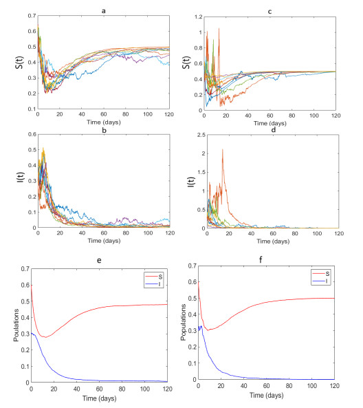
Epidemic models are used to understand the dynamics of disease transmission and explore the possible measures for preventing the spread of infection in the population. Disease transmission is intrinsically random and severely affected by environmental factors. We investigated a stochastic population model of the susceptible-infected-susceptible (SIS) type, in which infection spreads via both vertical and horizontal transmission routes. To incorporate stochasticity to the system, white multiplicative noise was taken into account in the horizontal disease transmission term. We proved that noise intensity, disease transmission, and recovery rates are potential routes for eradicating the disease. Furthermore, the parasite population reduces its fitness for some fixed noise if the relative fecundity of infected hosts and the disease transmission are low. However, if either of these is increased, it observes enhanced fitness. A simulation study illustrated the system's analytically dynamic properties and provided different insights. A case study for the imperfect vertical and horizontal infection transmission is also presented, supporting some of our observed theoretical results.
- stochastic population model,
- environmental factors,
- perfect and imperfect vertical transmissions,
- disease extinction time,
- persistence,
- stationary distribution,
- relative fecundity
Citation: Abhijit Majumder, Debadatta Adak, Adeline Samson, Nandadulal Bairagi. Persistence and extinction of infection in stochastic population model with horizontal and imperfect vertical disease transmissions[J]. Mathematical Biosciences and Engineering, 2025, 22(4): 846-875. doi: 10.3934/mbe.2025030

Related Papers:

Abstract

Epidemic models are used to understand the dynamics of disease transmission and explore the possible measures for preventing the spread of infection in the population. Disease transmission is intrinsically random and severely affected by environmental factors. We investigated a stochastic population model of the susceptible-infected-susceptible (SIS) type, in which infection spreads via both vertical and horizontal transmission routes. To incorporate stochasticity to the system, white multiplicative noise was taken into account in the horizontal disease transmission term. We proved that noise intensity, disease transmission, and recovery rates are potential routes for eradicating the disease. Furthermore, the parasite population reduces its fitness for some fixed noise if the relative fecundity of infected hosts and the disease transmission are low. However, if either of these is increased, it observes enhanced fitness. A simulation study illustrated the system's analytically dynamic properties and provided different insights. A case study for the imperfect vertical and horizontal infection transmission is also presented, supporting some of our observed theoretical results.

References

[1]	R. M. Anderson, R. M. May, The population dynamics of microparasites and their invertebrate hosts, Philos. Trans. R. Soc. B Biol. Sci., 291 (1981), 451–524. https://doi.org/10.1098/rstb.1981.0005 doi: 10.1098/rstb.1981.0005
[2]	M. Lipsitch, M. A. Nowak, D. Ebert, R. M. May, The population dynamics of vertically and horizontally transmitted parasites, Proc. R. Soc. B, 260 (1995), 321–327. https://doi.org/10.1098/rspb.1995.0099 doi: 10.1098/rspb.1995.0099
[3]	A. M. Dunn, J. E. Smith, Microsporidian life cycles and diversity: The relationship between virulence and transmission, Microbes Infect., 3 (2001), 381–388. https://doi.org/10.1016/S1286-4579(01)01394-6 doi: 10.1016/S1286-4579(01)01394-6
[4]	R. Fayer, Effect of high temperature on infectivity of Cryptosporidium parvum oocysts in water, Appl. Environ. Microbiol., 60 (1994), 2732–2735. https://doi.org/10.1128/aem.60.8.2732-2735.1994 doi: 10.1128/aem.60.8.2732-2735.1994
[5]	F. Memarzadeh, Literature review of the effect of temperature and humidity on viruses, ASHRAE Trans., 118 (2012), 1049–1060.
[6]	A. Gray, D. Greenhalgh, L. Hu, X. Mao, J. Pan, A stochastic differential equation SIS epidemic model, SIAM J. Appl. Math., 71 (2011), 876–902. https://doi.org/10.1137/10081856X doi: 10.1137/10081856X
[7]	Y. Zhao, D. Jiang, The threshold of a stochastic SIRS epidemic model with saturated incidence, Appl. Math. Lett., 34 (2014), 90–93. https://doi.org/10.1016/j.aml.2013.11.002 doi: 10.1016/j.aml.2013.11.002
[8]	A. Majumder, D. Adak, N. Bairagi, Phytoplankton-zooplankton interaction under environmental stochasticity: Survival, extinction and stability, Appl. Math. Model., 89 (2021), 1382–1404. https://doi.org/10.1016/j.apm.2020.06.076 doi: 10.1016/j.apm.2020.06.076
[9]	M. Lipsitch, S. Siller, M. A. Nowak, The evolution of virulence in pathogens with vertical and horizontal transmission, Evolution, 50 (1996), 1729–1741. https://doi.org/10.1111/j.1558-5646.1996.tb03560.x doi: 10.1111/j.1558-5646.1996.tb03560.x
[10]	Y. Chen, J. Evans, M. Feldlaufer, Horizontal and vertical transmission of viruses in the honey bee, Apis mellifera, J. Invertebr. Pathol., 92 (2006), 152–159. https://doi.org/10.1016/j.jip.2006.03.010 doi: 10.1016/j.jip.2006.03.010
[11]	D. H. Clayton, D. M. Tompkins, Ectoparasite virulence is linked to mode of transmission, Proc. R. Soc. B, 256 (1994), 211–217. https://doi.org/10.1098/rspb.1994.0072 doi: 10.1098/rspb.1994.0072
[12]	P. W. Ewald, Evolution of Infectious Disease, Oxford University Press on Demand, 1994.
[13]	J. Antonovics, A. J. Wilson, M. R. Forbes, H. C. Hauffe, E. R. Kallio, H. C. Leggett, et al., The evolution of transmission mode, Philos. Trans. R. Soc. B Biol. Sci., 372 (2017), 20160083. https://doi.org/10.1098/rstb.2016.0083 doi: 10.1098/rstb.2016.0083
[14]	N. Gao, Y. Song, X. Wang, J. Liu, Dynamics of a stochastic SIS epidemic model with nonlinear incidence rates, Adv. Contin. Discrete Models, 41 (2019), 1–19. https://doi.org/10.1186/s13662-019-1980-0 doi: 10.1186/s13662-019-1980-0
[15]	G. Lan, Y. Huang, C. Wei, S. Zhang, A stochastic SIS epidemic model with saturating contact rate, Phys. A Stat. Mech. Appl., 529 (2019), 121504. https://doi.org/10.1016/j.physa.2019.121504 doi: 10.1016/j.physa.2019.121504
[16]	A. Miao, T. Zhang, J. Zhang, C. Wang, Dynamics of a stochastic SIR model with both horizontal and vertical transmission, J. Appl. Anal. Comput., 8 (2018), 1108–1121. https://doi.org/10.11948/2018.1108 doi: 10.11948/2018.1108
[17]	D. Li, J. Cui, M. Liu, S. Liu, The evolutionary dynamics of stochastic epidemic model with nonlinear incidence rate, Bull. Math. Biol., 77 (2015), 1705–1743. https://doi.org/article/10.1007/s11538-015-0101-9 doi: 10.1007/s11538-015-0101-9
[18]	K. Mangin, M. Lipsitch, D. Ebert, Virulence and transmission modes of two microsporidia in Daphnia magna, Parasitology, 111 (2009), 133–142. https://doi.org/10.1017/S0031182000064878 doi: 10.1017/S0031182000064878
[19]	D. Ebert, M. Lipsitch, K. L. Mangin, The effect of parasites on host population density and extinction: Experimental epidemiology with Daphnia and six microparasites, Am. Nat., 156 (2000), 459–477. https://doi.org/10.1086/303404 doi: 10.1086/303404
[20]	R. E. Sorensen, D. J. Minchella, Parasite influences on host life history Echinostoma revolutum parasitism of Lymnaea elodes snails, Oecologia, 115 (1998), 188–195. https://doi.org/10.1007/s004420050507 doi: 10.1007/s004420050507
[21]	D. Tompkins, M. Begon, Parasites can regulate wildlife populations, Trends Parasitol., 15 (1999), 311–313. https://doi.org/10.1016/s0169-4758(99)01484-2 doi: 10.1016/s0169-4758(99)01484-2
[22]	J. C. HOLMES, Modification of intermediate host behaviour by parasites, Behav. Asp. Parasite Transm., (1972), 123–149. https://doi.org/10.5555/19730804260 doi: 10.5555/19730804260
[23]	K. D. Lafferty, A. K. Morris, Altered behavior of parasitized killifish increases susceptibility to predation by bird final hosts, Ecology, 77 (1996), 1390–1397. https://doi.org/10.2307/2265536 doi: 10.2307/2265536
[24]	P. Saha, N. Bairagi, Dynamics of vertically and horizontally transmitted parasites: Continuous vs discrete models, preprint, arXiv: 1906.03026. https://doi.org/10.48550/arXiv.1906.03026
[25]	N. C. Grassly, C. Fraser, Mathematical models of infectious disease transmission, Nat. Rev. Microbiol., 6 (2008), 477–487. https://doi.org/10.1038/nrmicro1845 doi: 10.1038/nrmicro1845
[26]	A. S. Mikhailov, A. Y. Loskutov, Foundations of Synergetics II: Complex Patterns, Springer Nature, 2012. https://link.springer.com/book/10.1007/978-3-642-80196-9
[27]	R. M. Anderson, B. Anderson, R. M. May, Infectious Diseases of Humans: Dynamics and Control, Oxford Academic, 1991. https://doi.org/10.1093/oso/9780198545996.001.0001
[28]	P. Van den Driessche, J. Watmough, Reproduction numbers and sub-threshold endemic equilibria for compartmental models of disease transmission, Math. Biosci., 180 (2002), 29–48. https://doi.org/10.1016/s0025-5564(02)00108-6 doi: 10.1016/s0025-5564(02)00108-6
[29]	N. Bairagi, D. Adak, Complex dynamics of a predator–prey–parasite system: An interplay among infection rate, predator's reproductive gain and preference, Ecol. Complex., 22 (2015), 1–12. https://doi.org/10.1016/j.ecocom.2015.01.002 doi: 10.1016/j.ecocom.2015.01.002
[30]	M. Kot, Elements of Mathematical Ecology, Cambridge University Press, 2001. https://doi.org/10.1017/CBO9780511608520
[31]	D. Valenti, A. Fiasconaro, B. Spagnolo, Stochastic resonance and noise delayed extinction in a model of two competing species, Phys. A Stat. Mech. Appl., 331 (2004), 477–486. https://doi.org/10.1016/j.physa.2003.09.036 doi: 10.1016/j.physa.2003.09.036
[32]	X. Mao, Stochastic Differential Equations and Applications, Elsevier, 2007.
[33]	M. Liu, K. Wang, Persistence and extinction in stochastic non-autonomous logistic systems, J. Math. Anal. Appl., 375 (2011), 443–457. https://doi.org/10.1016/j.jmaa.2010.09.058 doi: 10.1016/j.jmaa.2010.09.058
[34]	C. Ji, D. Jiang, Threshold behaviour of a stochastic SIR model, Appl. Math. Model., 38 (2014), 5067–5079. https://doi.org/10.1016/j.apm.2014.03.037 doi: 10.1016/j.apm.2014.03.037
[35]	V. V. Petrov, On the strong law of large numbers, Theory Probab. Appl., 14 (1969), 183–192. https://doi.org/10.1137/1114027 doi: 10.1137/1114027
[36]	R. M. May, Stability and Complexity in Model Ecosystems, Princeton University Press, 2019. https://doi.org/10.2307/j.ctvs32rq4
[37]	S. Olaniyi, O. S. Obabiyi, Qualitative analysis of malaria dynamics with nonlinear incidence function, Appl. Math. Sci., 8 (2014), 3889–3904. http://dx.doi.org/10.12988/ams.2014.45326 doi: 10.12988/ams.2014.45326
[38]	S. Mushayabasa, C. Bhunu, Modeling HIV transmission dynamics among male prisoners in sub-saharan africa, Int. J. Appl. Math., 41 (2011).
[39]	I. M. Sobol, Global sensitivity indices for nonlinear mathematical models and their monte carlo estimates, Math. Comput. Simul., 55 (2001), 271–280. https://doi.org/10.1016/S0378-4754(00)00270-6 doi: 10.1016/S0378-4754(00)00270-6
[40]	O. Kaltz, J. C. Koella, Host growth conditions regulate the plasticity of horizontal and vertical transmission in Holospora undulata, a bacterial parasite of the protozoan paramecium caudatum, Evolution, 57 (2003), 1535–1542. https://doi.org/10.1111/j.0014-3820.2003.tb00361.x doi: 10.1111/j.0014-3820.2003.tb00361.x
[41]	D. Lunn, R. J. Goudie, C. Wei, O. Kaltz, O. Restif, Modelling the dynamics of an experimental host-pathogen microcosm within a hierarchical Bayesian framework, PLOS One, 8 (2013), e69775. https://doi.org/10.1371/journal.pone.0069775 doi: 10.1371/journal.pone.0069775
[42]	W. O. Kermack, A. G. McKendrick, A contribution to the mathematical theory of epidemics, Proc. R. Soc. Lond. A, 115 (1927), 700–721. https://doi.org/10.1098/rspa.1927.0118 doi: 10.1098/rspa.1927.0118
[43]	M. Liu, K. Wang, Global stability of a nonlinear stochastic predator-prey system with Beddington-DeAngelis functional response, Commun. Nonlinear Sci. Numer. Simul., 16 (2011), 1114–1121. https://doi.org/10.1016/j.cnsns.2010.06.015 doi: 10.1016/j.cnsns.2010.06.015
[44]	S. Liu, Y. Pei, C. Li, L. Chen, Three kinds of TVS in a SIR epidemic model with saturated infectious force and vertical transmission, Appl. Math. Model., 33 (2009), 1923–1932. https://doi.org/10.1016/j.apm.2008.05.001 doi: 10.1016/j.apm.2008.05.001
[45]	J. Tanimoto, Sociophysics Approach to Epidemics, Springer, 23 (2021). https://link.springer.com/book/10.1007/978-981-33-6481-3
[46]	B. Zhou, D. Jiang, B. Han, T. Hayat, Threshold dynamics and density function of a stochastic epidemic model with media coverage and mean-reverting Ornstein-Uhlenbeck process, Math. Comput. Simul., 196 (2022), 15–44. https://doi.org/10.1016/j.matcom.2022.01.014 doi: 10.1016/j.matcom.2022.01.014
[47]	E. Allen, Environmental variability and mean-reverting processes, Discrete Contin. Dyn. Syst. Ser. B, 21 (2016), 2073–2089. https://www.aimsciences.org/article/doi/10.3934/dcdsb.2016037
[48]	K. Mamis, M. Farazmand, Stochastic compartmental models of the Covid-19 pandemic must have temporally correlated uncertainties, Proc. R. Soc. A, 479 (2023), 20220568. https://doi.org/10.1098/rspa.2022.0568 doi: 10.1098/rspa.2022.0568
[49]	K. Mamis, M. Farazmand, Modeling correlated uncertainties in stochastic compartmental models, Math. Biosci., 374 (2024), 109226. https://doi.org/10.1016/j.mbs.2024.109226 doi: 10.1016/j.mbs.2024.109226
[50]	J. Nocedal, S. J. Wright, Numerical optimization, 2nd edition, Springer, New York, 2006.
[51]	M. I. Lourakis, A brief description of the Levenberg-Marquardt algorithm implemented by levmar, Foundation Res. Technol., 4 (2005), 1–6. http://www.ics.forth.gr/lourakis/levmar

Reader Comments

Your name:*

Email:*
© 2025 the Author(s), licensee AIMS Press. This is an open access article distributed under the terms of the Creative Commons Attribution License (http://creativecommons.org/licenses/by/4.0)