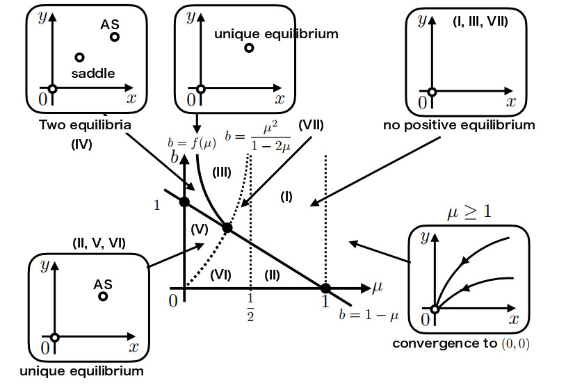
There are known methods to manage the population dynamics of wild and sterile mosquitoes by releasing genetically engineered sterile mosquitoes. Even if a two-dimensional system of ordinary differential equations is considered as a simple mathematical model for developing release strategies, fully understanding the global behavior of the solutions is challenging, due to the fact that the probability of mating is ratio-dependent. In this paper, we combine a geometric approach called the time-scale transformation and blow-up technique with the center manifold theorem to provide a complete understanding of dynamical systems near the origin. Then, the global behavior of the solution of the two-dimensional ordinary differential equation system is classified in a two-parameter plane represented by the natural death rate of mosquitoes and the sterile mosquito release rate. We also offer a discussion of the sterile mosquito release strategy. In addition, we obtain a better exposition of the previous results on the existence and local stability of positive equilibria. This paper provides a framework for the mathematical analysis of models with ratio-dependent terms, and we expect that it will theoretically withstand the complexity of improved models.
Citation: Yu Ichida, Yukihiko Nakata. Global dynamics of a simple model for wild and sterile mosquitoes[J]. Mathematical Biosciences and Engineering, 2024, 21(9): 7016-7039. doi: 10.3934/mbe.2024308
There are known methods to manage the population dynamics of wild and sterile mosquitoes by releasing genetically engineered sterile mosquitoes. Even if a two-dimensional system of ordinary differential equations is considered as a simple mathematical model for developing release strategies, fully understanding the global behavior of the solutions is challenging, due to the fact that the probability of mating is ratio-dependent. In this paper, we combine a geometric approach called the time-scale transformation and blow-up technique with the center manifold theorem to provide a complete understanding of dynamical systems near the origin. Then, the global behavior of the solution of the two-dimensional ordinary differential equation system is classified in a two-parameter plane represented by the natural death rate of mosquitoes and the sterile mosquito release rate. We also offer a discussion of the sterile mosquito release strategy. In addition, we obtain a better exposition of the previous results on the existence and local stability of positive equilibria. This paper provides a framework for the mathematical analysis of models with ratio-dependent terms, and we expect that it will theoretically withstand the complexity of improved models.

| [1] | V. A. Dyck, J. Hendrichs, A. S. Robinson, Sterile insect technique: principles and practice in area-wide integrated pest management, Taylor, Francis, 2021. https://doi.org/10.1201/9781003035572 |
| [2] |
R. Anguelov, Y. Dumont, J. Lubuma, Mathematical modeling of sterile insect technology for control of anopheles mosquito, Comput. Math. Appl., 64 (2012), 374–389. https://doi.org/10.1016/j.camwa.2012.02.068 doi: 10.1016/j.camwa.2012.02.068

|
| [3] |
R. Anguelov, Y. Dumont, I. V. Y. Djeumen, Sustainable vector/pest control using the permanent sterile insect technique, Math. Methods Appl. Sci., 43 (2020), 10391–10412. https://doi.org/10.1002/mma.6385 doi: 10.1002/mma.6385
|
| [4] |
M. Aronna, Y. Dumont, On nonlinear pest/vector control via the sterile insect technique: impact of residual fertility, Bull. Math. Biol., 110 (2020), 29. https://doi.org/10.1007/s11538-020-00790-3 doi: 10.1007/s11538-020-00790-3
|
| [5] |
P. A. Bliman, D. Cardona-Salgado, Y. Dumont, O. Vasilieva, Implementation of control strategies for sterile insect techniques, Math. Biosci., 314 (2019), 43–60. https://doi.org/10.1016/j.mbs.2019.06.002 doi: 10.1016/j.mbs.2019.06.002
|
| [6] |
L. Cai, S. Ai, J. Li, Dynamics of mosquitoes populations with different strategies for releasing sterile mosquitoes, SIAM J. Appl. Math., 74 (2014), 1786–1809. https://doi.org/10.1137/13094102X doi: 10.1137/13094102X
|
| [7] |
Y. Dumont, C. F. Oliva, On the impact of re-mating and residual fertility on the sterile insect technique efficacy: Case study with the medfly, ceratitis capitata, PLOS Comput. Biol., 20 (2024), 1–35. https://doi.org/10.1371/journal.pcbi.1012052 doi: 10.1371/journal.pcbi.1012052
|
| [8] |
Y. Dumont, I. Yatat-Djeumen, About contamination by sterile females and residual male fertility on the effectiveness of the sterile insect technique, impact on disease vector control and disease control, Math. Biosci., 370 (2024), 109–165. https://doi.org/10.1016/j.mbs.2024.109165 doi: 10.1016/j.mbs.2024.109165
|
| [9] |
J. Li, New revised simple models for interactive wild and sterile mosquito populations and their dynamics, J. Biol. Dyn. 11 (2017), 79–101. https://doi.org/10.1080/17513758.2016.1216613 doi: 10.1080/17513758.2016.1216613
|
| [10] |
J. Li, L. Cai, Y. Li Stage-structured wild and sterile mosquito population models and their dynamics, J. Biol. Dyn. S1 (2016), 79–101. https://doi.org/10.1080/17513758.2016.1159740 doi: 10.1080/17513758.2016.1159740
|
| [11] |
J. Li, Z. Yuan Modelling releases of sterile mosquitoes with different strategies, J. Biol. Dyn., 9 (2015), 1–14. https://doi.org/10.1080/17513758.2014.977971 doi: 10.1080/17513758.2014.977971
|
| [12] |
S. K. Sasmal, Y. Takeuchi, Y. Nakata, A simple model to control the wild mosquito with sterile release, J. Math. Anal. Appl. 531 (2024), 127828. https://doi.org/10.1016/j.jmaa.2023.127828 doi: 10.1016/j.jmaa.2023.127828
|
| [13] |
M. Strugarek, H. Bossin, Y. Dumont, On the use of the sterile insect technique or the incompatible insect technique to reduce or eliminate mosquito populations, Appl. Math. Model., 68 (2019), 443–470. https://doi.org/10.48550/arXiv.1805.10150 doi: 10.48550/arXiv.1805.10150
|
| [14] |
D. Xiao, S. Ruan, Global dynamics of a ratio-dependent predator-prey system, J. Math. Biol., 43 (2001), 268–290. https://doi.org/10.1007/s002850100097 doi: 10.1007/s002850100097
|
| [15] |
M. J. Álvarez, A. Ferragut, X. Jarque, A survey on the blow up technique, Int. J. Bifurc. Chaos, 21 (2021), 3108–3118. https://doi.org/10.1142/S0218127411030416 doi: 10.1142/S0218127411030416
|
| [16] |
M. Brunella, M, Miari, Topological equivalence of a plane vector field with its principal part defined through Newton polyhedra, J. Differ. Equations, 85 (1990), 338–366. https://doi.org/10.1016/0022-0396(90)90120-E doi: 10.1016/0022-0396(90)90120-E
|
| [17] | F. Dumortier, J. Llibre, C. J. Artés, Qualitative Theory of Planar Differential Systems, Springer, 2006. |
| [18] | C. Kuehn, Multiple Time Scale Dynamics, Springer, 2015. |
| [19] | J. Carr, Applications of Centre Manifold Theory, Springer-Verlag, New York-Berlin, 1981. |
| [20] | S. Wiggins, Introduction to Applied Nonlinear Dynamical Systems and Chaos, Springer-Verlag, New York, 2003. |


Figures(6)

Yu Ichida, Yukihiko Nakata. Global dynamics of a simple model for wild and sterile mosquitoes[J]. Mathematical Biosciences and Engineering, 2024, 21(9): 7016-7039. doi: 10.3934/mbe.2024308


 DownLoad: